gnuplot
系列教程:
http://blog.sciencenet.cn/blog-373392-518247.html
基本环境
命令gnuplot启动repl交互:
$ gnuplot

        G N U P L O T
        Version 4.6 patchlevel 4    last modified 2013-10-02
        Build System: Linux x86_64

        Copyright (C) 1986-1993, 1998, 2004, 2007-2013
        Thomas Williams, Colin Kelley and many others

        gnuplot home:     http://www.gnuplot.info
        faq, bugs, etc:   type "help FAQ"
        immediate help:   type "help"  (plot window: hit 'h')

Terminal type set to 'wxt'
gnuplot>
执行再有的脚本:
gnuplot> load 'plot.plt'
调用系统命令:
!vim plot.plt
绘制二维图像
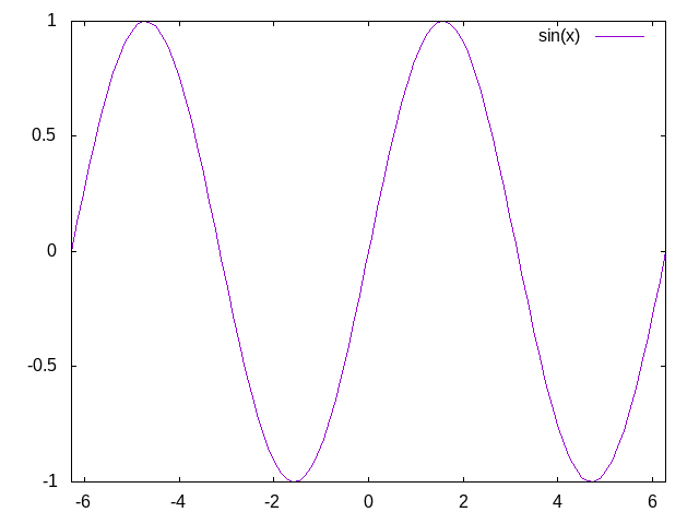
plot指令可以用来绘制二维图像:
plot sin(x) linewidth 4
-
help plot查看帮助信息。 -
linewidth指定函数线条的粗细。 -
笛卡尔坐标系下默认的变量名为
x,默认的范围在\(-10 ~ 10\)。 -
如果变量名不用
x的话会报错,如plot sin(y)就报错「undefined varible: y」
保存图像
set term png              # 定义图像格式
set output "sin.png"      # 保存的文件名
plot sin(x)
查看所有支持的格式:
gnuplot> set term

Available terminal types:
       cairolatex  LaTeX picture environment using graphicx package and Cairo backend
           canvas  HTML Canvas object
              cgm  Computer Graphics Metafile
          context  ConTeXt with MetaFun (for PDF documents)
            corel  EPS format for CorelDRAW
             dumb  ascii art for anything that prints text
              dxf  dxf-file for AutoCad (default size 120x80)
            eepic  EEPIC -- extended LaTeX picture environment
              emf  Enhanced Metafile format
            emtex  LaTeX picture environment with emTeX specials
         epscairo  eps terminal based on cairo
         epslatex  LaTeX picture environment using graphicx package
              fig  FIG graphics language for XFIG graphics editor
              gif  GIF images using libgd and TrueType fonts
             gpic  GPIC -- Produce graphs in groff using the gpic preprocessor
          hp2623A  HP2623A and maybe others
           hp2648  HP2648 and HP2647
             hpgl  HP7475 and relatives [number of pens] [eject]
           imagen  Imagen laser printer
             jpeg  JPEG images using libgd and TrueType fonts
            latex  LaTeX picture environment
Press return for more:
一般LaTeX中使用eps或是epslatex比较常见:
set term postscript
set output "sin.eps"
Gnuplot基本程序结构
# Bipolar Transistor (NPN) Mutual Characteristic  # comment

Ie(Vbe) = Ies*exp(Vbe/kT_q)                       # defined functions
Ic(Vbe) = alpha*Ie(Vbe)+Ico                       # and constants
alpha   = 0.99
Ies     = 4e-14
Ico     = 1e-09
kT_q    = 0.025

set dummy Vbe                                     # set plotting environment
set grid
set samples 160
set title  "Mutual Characteristic of a Transistor"
set xlabel "Vbe (base emmitter voltage)"
set xrange [0 : 0.75]
set ylabel "Ic (collector current)"
set yrange [0 : 0.005]
# set key 0.2,0.0045
set format y "%.4f"

plot Ic(Vbe)                                      # plotting

set terminal postscript                           # output
set output "npn.ps"
replot
图像设置
设置图像大小
set term png size 600,400
字体设置
set term png size 600,400 enhanced font "Sans"
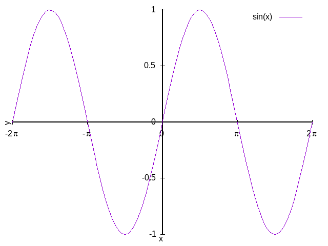
选项enhanced可以用来显示特殊符号,比如「\(\pi\)」
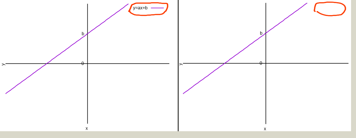
标题设置
set title 'sketch of sine function'
边框设置
unset border # 不显示外框
显示图例
set key off
配置坐标轴
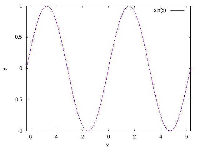
设置范围
设置\(x\)轴\(y\)轴的范围:
set xrange [-2*pi : 2*pi]
set yrange [-1 : 1]

plot sin(x) title "sin(x)"
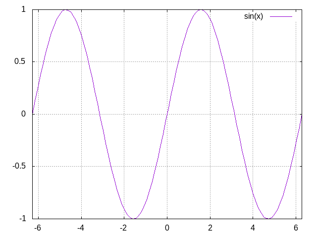
设置网络
set grid xtics
set grid ytics
设置标签
设置\(x\)轴与\(y\)轴的标注:
set xlabel "x"
set ylabel "y"
设置刻度
默认刻度
默认刻度会平均刻度的间距。
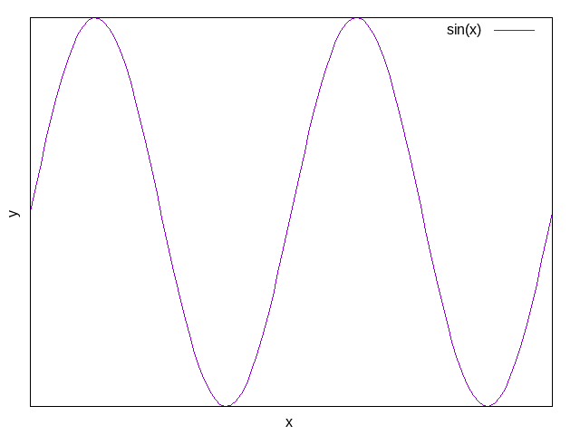
不显示刻度
unset xtics
unset ytics
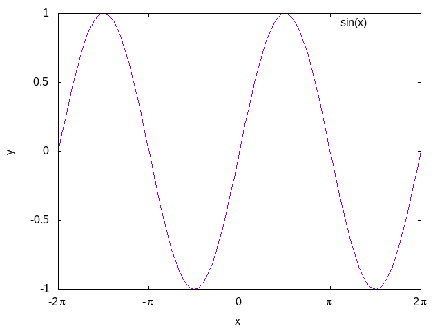
指定刻度
格式一:每一个刻度的值和标题
set xtics ('-2{/Symbol p}' -2 * pi, '-{/Symbol p}' -pi, '0' 0, '{/Symbol p}' pi, '2{/Symbol p}' 2 * pi)

格式二:最小,步长,最大
set ytics -1, 0.5, 1
不显示外框
unset border # 不显示外框
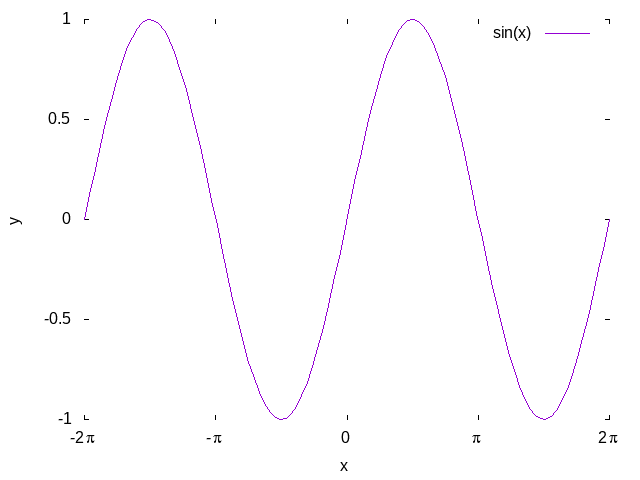
显示X轴与Y轴
set zeroaxis lt -1 lw 2   # 画出X轴与Y轴
set xtics axis ('-2{/Symbol p}' -2 * pi, '-{/Symbol p}' -pi, '0' 0, '{/Symbol p}' pi, '2{/Symbol p}' 2 * pi)
set ytics axis -1, 0.5, 1
绘制函数
支持的函数
__________________________________________________________
Function            Returns
-----------      ------------------------------------------
abs(x)            absolute value of x, |x|
acos(x)           arc-cosine  of x
asin(x)           arc-sine    of x
atan(x)           arc-tangent of x
cos(x)            cosine      of x,  x is in radians.
cosh(x)           hyperbolic cosine of x, x is in radians
erf(x)            error function of x
exp(x)            exponential function of x, base e
inverf(x)         inverse error function of x
invnorm(x)        inverse normal distribution of x
log(x)            log of x, base e
log10(x)          log of x, base 10
norm(x)           normal Gaussian distribution function
rand(x)           pseudo-random number generator
sgn(x)            1 if x > 0, -1 if x < 0, 0 if x=0
sin(x)            sine      of x, x is in radians
sinh(x)           hyperbolic sine of x, x is in radians
sqrt(x)           the square root of x
tan(x)            tangent of x, x is in radians
tanh(x)           hyperbolic tangent of x, x is in radians
___________________________________________________________
Bessel, gamma, ibeta, igamma, and lgamma functions are also
supported.  Many functions can take complex arguments.
Binary and unary operators are also supported.
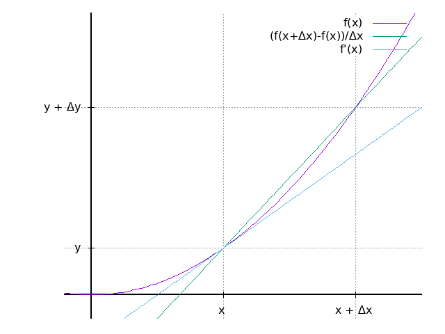
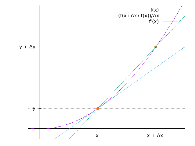
绘制多个函数
plot x**2    title "f(x)" , \
     3*x - 2 title "(f(x+{/symbol D}x)-f(x))/{/symbol D}x" , \
     2*x - 1 title "f'(x)"
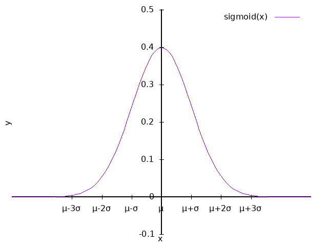
定义常量
e=2.7182818284
mu = 0
sgm = 1

x0 = mu - 3*sgm
x1 = mu - 2*sgm
x2 = mu - sgm
x3 = mu
x4 = mu + sgm
x5 = mu + 2*sgm
x6 = mu + 3*sgm

# 坐标轴上的刻度  σ μ
set xtics axis ( \
		"μ{/symbol m}-3{/symbol s}" x0,  \
		"{/symbol m}-2{/symbol s}" x1,   \
		"{/symbol m}-{/symbol s}" x2,    \
		"{/symbol m}"x3,                 \
		"{/symbol m}+{/symbol s}" x4,    \
		"{/symbol m}+2{/symbol s}" x5,   \
		"{/symbol m}+3{/symbol s}" x6)
set ytics axis

plot 1/(sqrt(2 * pi) * sgm) * e ** (-1 * (x - mu)**2 / (2 * sgm**2)) \
     title "sigmoid(x)"
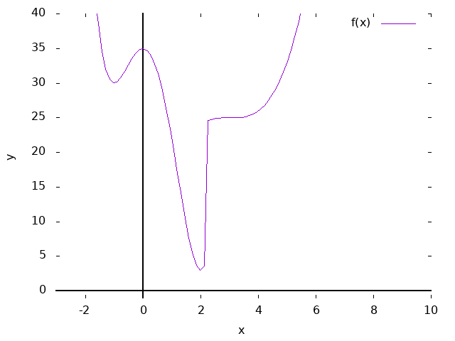
定义函数
f(x)= x>2.2 && x<10   ? \
      (x-3) ** 3 + 25 : \
      3*x**4 - 4*x**3 - 12*x**2 + 35
plot f(x)
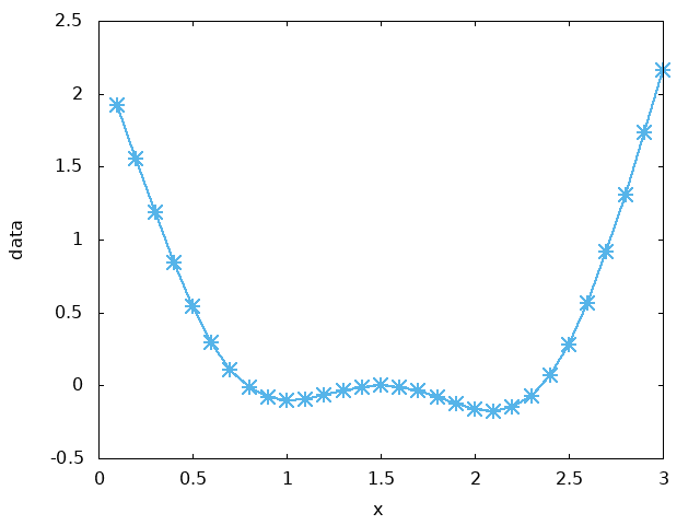
从数据文件绘制图形
数据文件data.dat:
0.1                               1.9209304925688333
0.2                               1.556593079864876
0.30000000000000004               1.1884832854699365
0.4                               0.8430151183100703
0.5                               0.5403023058681398
0.6000000000000001                0.2935097811261054
0.7000000000000001                0.1087789714561541
0.8                               -0.014307765927631517
0.9                               -0.08179275408951135
1.0                               -0.1040367091367856
1.1                               -0.09416017876085528
1.2000000000000002                -0.06636543439871205
1.3                               -0.03427555013475787
1.4000000000000001                -0.009422223406686558
1.5                               -0.0
1.6                               -0.00998294775794755
1.7000000000000002                -0.0386719277031785
1.8                               -0.08070825747007325
1.9000000000000001                -0.12655483390630673
2.0                               -0.16341090521590299
2.1                               -0.17649389568265184
2.2                               -0.15059310628942557
2.3000000000000003                -0.07177761723843461
2.4000000000000004                0.07087417658595234
2.5                               0.28366218546322625
2.6                               0.5669051722734564
2.7                               0.9139577413573942
2.8000000000000003                1.3107063346823233
2.9000000000000004                1.7356182532049869
3.0                               2.1603831449633235
使用linespoints画图,线宽2.5、线的类型为3:
set xlabel "x"
set ylabel "data"
set pointsize 2.0

plot 'data.dat' with linespoints linewidth 2.5 linetype 3 notitle
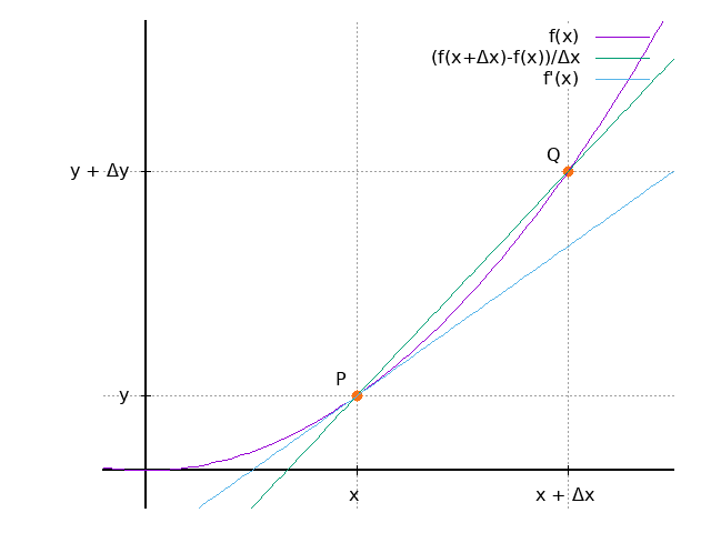
绘标注
标注点
set label 1 at 1,1 point pt 7 ps 1.5 lc rgb "#F87217"
set label 3 at 2,4 point pt 7 ps 1.5 lc rgb "#F87217"
文字描述
set label 2 "P" at 0.9,1.2
set label 4 "Q" at 1.9,4.2
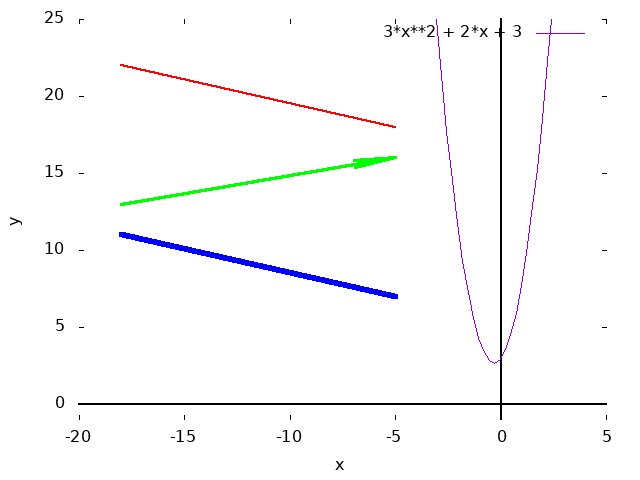
箭头与线段
set arrow 1 from -18,22 to -5,18 nofilled size 0.1,0.1,0.1 lc rgb "#ff0000" lw 2
set arrow 2 from -18,13 to -5,16 nofilled size 2.0,5.0,5.0 lc rgb "#00ff00" lw 3
set arrow 3 from -18,11 to -5,7  nofilled size 0.1,0.1,0.1 lc rgb "#0000ff" lw 5
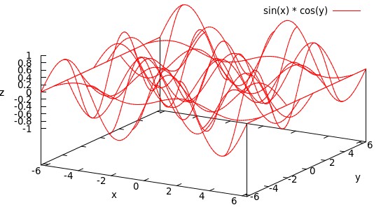
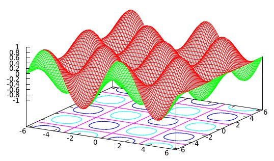
绘制三维图像
splot命令用来绘制三维图像,两个变量分别是x和y:
set xrange [-2 * pi : 2 * pi]
set yrange [-2 * pi : 2 * pi]
splot sin(x) * sin(y)
定义等值线的密度
set isosamples 75, 75
replot
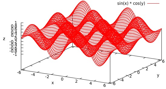
隐藏三维图像的背面线条
隐藏背面的线条:
set hidden3d
replot
调整Z轴
把z轴的零点移到xy平面上:
set ticslevel 0
replot
调整观察角度
gnuplot窗口中显示的3维图像可以用鼠标调整角度。
如果输出是文件,可以用set view定义角度,四个参数的意义请查看手册。
set view *, *, *, *
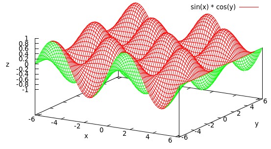
等高线
因为没有专门的等高线命令,所以还是使用splot二维绘制实现:
set xrange [-2 * pi : 2 * pi]
set yrange [-2 * pi : 2 * pi]
set isosamples 100,100
set hidden3d

set contour base           # 在底部显示等高线
splot sin(x) * cos(y) notitle
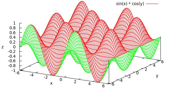
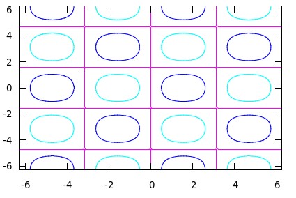
调整只显示等高线:
unset surface    # 不显示三维部分,只显示等高线
set view map     # 以map角度观察图像
set key out      # 在图像杠外显示图例
replot
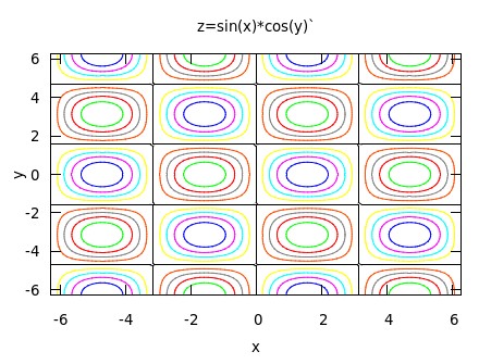
把等高线的设置得更加密致:
set cntrparam levels discrete -0.8, -0.6, -0.4, -0.2, 0, 0.2, 0.4, 0.6, 0.8
set xlabel 'x'
set ylabel 'y'
set title 'z=sin(x)*cos(y)`
replot
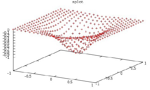
从数据文件绘制三维视图
0.1     0.1     0.01999999999999999
0.1     0.2     0.02999999999999997
0.1     0.30000000000000004     -0.020000000000000018
0.1     0.4     -0.13000000000000006
0.1     0.5     -0.3
0.1     0.6000000000000001     -0.5300000000000002
0.1     0.7000000000000001     -0.8200000000000002
0.1     0.8     -1.1700000000000004
0.1     0.9     -1.58
0.1     1.0     -2.05
0.1     1.1     -2.580000000000001
0.1     1.2000000000000002     -3.170000000000001
0.1     1.3     -3.8200000000000003
0.1     1.4000000000000001     -4.530000000000001
0.1     1.5     -5.3
0.1     1.6     -6.130000000000002
0.1     1.7000000000000002     -7.020000000000001
0.1     1.8     -7.970000000000001
0.1     1.9000000000000001     -8.980000000000002
0.1     2.0     -10.05
0.1     2.1     -11.18
0.2     0.1     -0.13000000000000003
0.2     0.2     -0.12000000000000005
0.2     0.30000000000000004     -0.17000000000000007
0.2     0.4     -0.28000000000000014
0.2     0.5     -0.45000000000000007
0.2     0.6000000000000001     -0.6800000000000003
0.2     0.7000000000000001     -0.9700000000000002
0.2     0.8     -1.3200000000000003
0.2     0.9     -1.7300000000000002
0.2     1.0     -2.2
0.2     1.1     -2.730000000000001
0.2     1.2000000000000002     -3.320000000000001
0.2     1.3     -3.97
0.2     1.4000000000000001     -4.680000000000001
0.2     1.5     -5.45
0.2     1.6     -6.280000000000001
0.2     1.7000000000000002     -7.170000000000002
0.2     1.8     -8.120000000000001
0.2     1.9000000000000001     -9.130000000000003
0.2     2.0     -10.2
0.2     2.1     -11.33
0.30000000000000004     0.1     -0.3800000000000001
0.30000000000000004     0.2     -0.3700000000000001
0.30000000000000004     0.30000000000000004     -0.42000000000000015
0.30000000000000004     0.4     -0.5300000000000002
0.30000000000000004     0.5     -0.7000000000000002
0.30000000000000004     0.6000000000000001     -0.9300000000000004
0.30000000000000004     0.7000000000000001     -1.2200000000000002
0.30000000000000004     0.8     -1.5700000000000005
0.30000000000000004     0.9     -1.9800000000000002
0.30000000000000004     1.0     -2.45
0.30000000000000004     1.1     -2.980000000000001
0.30000000000000004     1.2000000000000002     -3.570000000000001
0.30000000000000004     1.3     -4.220000000000001
0.30000000000000004     1.4000000000000001     -4.930000000000001
0.30000000000000004     1.5     -5.7
0.30000000000000004     1.6     -6.530000000000001
0.30000000000000004     1.7000000000000002     -7.420000000000002
0.30000000000000004     1.8     -8.370000000000001
0.30000000000000004     1.9000000000000001     -9.380000000000003
0.30000000000000004     2.0     -10.45
0.30000000000000004     2.1     -11.58
0.4     0.1     -0.7300000000000002
0.4     0.2     -0.7200000000000001
0.4     0.30000000000000004     -0.7700000000000002
0.4     0.4     -0.8800000000000002
0.4     0.5     -1.0500000000000003
0.4     0.6000000000000001     -1.2800000000000002
0.4     0.7000000000000001     -1.5700000000000003
0.4     0.8     -1.9200000000000004
0.4     0.9     -2.33
0.4     1.0     -2.8000000000000003
0.4     1.1     -3.330000000000001
0.4     1.2000000000000002     -3.9200000000000013
0.4     1.3     -4.57
0.4     1.4000000000000001     -5.280000000000001
0.4     1.5     -6.05
0.4     1.6     -6.880000000000002
0.4     1.7000000000000002     -7.770000000000001
0.4     1.8     -8.72
0.4     1.9000000000000001     -9.730000000000002
0.4     2.0     -10.8
0.4     2.1     -11.93
0.5     0.1     -1.18
0.5     0.2     -1.1700000000000002
0.5     0.30000000000000004     -1.22
0.5     0.4     -1.33
0.5     0.5     -1.5
0.5     0.6000000000000001     -1.7300000000000002
0.5     0.7000000000000001     -2.02
0.5     0.8     -2.37
0.5     0.9     -2.7800000000000002
0.5     1.0     -3.25
0.5     1.1     -3.7800000000000007
0.5     1.2000000000000002     -4.370000000000001
0.5     1.3     -5.0200000000000005
0.5     1.4000000000000001     -5.73
0.5     1.5     -6.5
0.5     1.6     -7.330000000000002
0.5     1.7000000000000002     -8.220000000000002
0.5     1.8     -9.17
0.5     1.9000000000000001     -10.180000000000001
0.5     2.0     -11.25
0.5     2.1     -12.38
0.6000000000000001     0.1     -1.7300000000000004
0.6000000000000001     0.2     -1.7200000000000006
0.6000000000000001     0.30000000000000004     -1.7700000000000005
0.6000000000000001     0.4     -1.8800000000000003
0.6000000000000001     0.5     -2.0500000000000007
0.6000000000000001     0.6000000000000001     -2.2800000000000007
0.6000000000000001     0.7000000000000001     -2.5700000000000007
0.6000000000000001     0.8     -2.920000000000001
0.6000000000000001     0.9     -3.3300000000000005
0.6000000000000001     1.0     -3.8000000000000007
0.6000000000000001     1.1     -4.330000000000001
0.6000000000000001     1.2000000000000002     -4.920000000000002
0.6000000000000001     1.3     -5.57
0.6000000000000001     1.4000000000000001     -6.280000000000001
0.6000000000000001     1.5     -7.050000000000001
0.6000000000000001     1.6     -7.880000000000002
0.6000000000000001     1.7000000000000002     -8.770000000000001
0.6000000000000001     1.8     -9.72
0.6000000000000001     1.9000000000000001     -10.730000000000002
0.6000000000000001     2.0     -11.8
0.6000000000000001     2.1     -12.930000000000001
0.7000000000000001     0.1     -2.3800000000000003
0.7000000000000001     0.2     -2.3700000000000006
0.7000000000000001     0.30000000000000004     -2.4200000000000004
0.7000000000000001     0.4     -2.5300000000000007
0.7000000000000001     0.5     -2.7000000000000006
0.7000000000000001     0.6000000000000001     -2.9300000000000006
0.7000000000000001     0.7000000000000001     -3.2200000000000006
0.7000000000000001     0.8     -3.570000000000001
0.7000000000000001     0.9     -3.980000000000001
0.7000000000000001     1.0     -4.450000000000001
0.7000000000000001     1.1     -4.980000000000001
0.7000000000000001     1.2000000000000002     -5.570000000000002
0.7000000000000001     1.3     -6.220000000000001
0.7000000000000001     1.4000000000000001     -6.9300000000000015
0.7000000000000001     1.5     -7.700000000000001
0.7000000000000001     1.6     -8.530000000000001
0.7000000000000001     1.7000000000000002     -9.420000000000002
0.7000000000000001     1.8     -10.370000000000001
0.7000000000000001     1.9000000000000001     -11.380000000000003
0.7000000000000001     2.0     -12.450000000000001
0.7000000000000001     2.1     -13.580000000000002
0.8     0.1     -3.1300000000000003
0.8     0.2     -3.1200000000000006
0.8     0.30000000000000004     -3.1700000000000004
0.8     0.4     -3.2800000000000007
0.8     0.5     -3.4500000000000006
0.8     0.6000000000000001     -3.6800000000000006
0.8     0.7000000000000001     -3.9700000000000006
0.8     0.8     -4.32
0.8     0.9     -4.73
0.8     1.0     -5.200000000000001
0.8     1.1     -5.730000000000001
0.8     1.2000000000000002     -6.320000000000002
0.8     1.3     -6.970000000000001
0.8     1.4000000000000001     -7.6800000000000015
0.8     1.5     -8.450000000000001
0.8     1.6     -9.280000000000001
0.8     1.7000000000000002     -10.170000000000002
0.8     1.8     -11.120000000000001
0.8     1.9000000000000001     -12.130000000000003
0.8     2.0     -13.200000000000001
0.8     2.1     -14.330000000000002
0.9     0.1     -3.9800000000000004
0.9     0.2     -3.9700000000000006
0.9     0.30000000000000004     -4.020000000000001
0.9     0.4     -4.130000000000001
0.9     0.5     -4.300000000000001
0.9     0.6000000000000001     -4.530000000000001
0.9     0.7000000000000001     -4.82
0.9     0.8     -5.170000000000002
0.9     0.9     -5.580000000000001
0.9     1.0     -6.050000000000001
0.9     1.1     -6.580000000000002
0.9     1.2000000000000002     -7.170000000000002
0.9     1.3     -7.820000000000001
0.9     1.4000000000000001     -8.530000000000001
0.9     1.5     -9.3
0.9     1.6     -10.130000000000003
0.9     1.7000000000000002     -11.020000000000003
0.9     1.8     -11.970000000000002
0.9     1.9000000000000001     -12.980000000000002
0.9     2.0     -14.05
0.9     2.1     -15.180000000000001
1.0     0.1     -4.930000000000001
1.0     0.2     -4.92
1.0     0.30000000000000004     -4.970000000000001
1.0     0.4     -5.08
1.0     0.5     -5.25
1.0     0.6000000000000001     -5.48
1.0     0.7000000000000001     -5.77
1.0     0.8     -6.120000000000001
1.0     0.9     -6.529999999999999
1.0     1.0     -7.0
1.0     1.1     -7.530000000000001
1.0     1.2000000000000002     -8.120000000000001
1.0     1.3     -8.77
1.0     1.4000000000000001     -9.48
1.0     1.5     -10.25
1.0     1.6     -11.080000000000002
1.0     1.7000000000000002     -11.970000000000002
1.0     1.8     -12.920000000000002
1.0     1.9000000000000001     -13.930000000000001
1.0     2.0     -15.0
1.0     2.1     -16.13
1.1     0.1     -5.980000000000001
1.1     0.2     -5.970000000000001
1.1     0.30000000000000004     -6.020000000000001
1.1     0.4     -6.130000000000001
1.1     0.5     -6.300000000000001
1.1     0.6000000000000001     -6.530000000000001
1.1     0.7000000000000001     -6.82
1.1     0.8     -7.170000000000002
1.1     0.9     -7.58
1.1     1.0     -8.05
1.1     1.1     -8.580000000000002
1.1     1.2000000000000002     -9.170000000000002
1.1     1.3     -9.82
1.1     1.4000000000000001     -10.530000000000001
1.1     1.5     -11.3
1.1     1.6     -12.130000000000003
1.1     1.7000000000000002     -13.020000000000003
1.1     1.8     -13.970000000000002
1.1     1.9000000000000001     -14.980000000000002
1.1     2.0     -16.05
1.1     2.1     -17.18
1.2000000000000002     0.1     -7.130000000000003
1.2000000000000002     0.2     -7.120000000000002
1.2000000000000002     0.30000000000000004     -7.170000000000003
1.2000000000000002     0.4     -7.280000000000002
1.2000000000000002     0.5     -7.450000000000002
1.2000000000000002     0.6000000000000001     -7.6800000000000015
1.2000000000000002     0.7000000000000001     -7.970000000000002
1.2000000000000002     0.8     -8.320000000000002
1.2000000000000002     0.9     -8.730000000000002
1.2000000000000002     1.0     -9.200000000000003
1.2000000000000002     1.1     -9.730000000000002
1.2000000000000002     1.2000000000000002     -10.320000000000004
1.2000000000000002     1.3     -10.970000000000002
1.2000000000000002     1.4000000000000001     -11.680000000000003
1.2000000000000002     1.5     -12.450000000000003
1.2000000000000002     1.6     -13.280000000000003
1.2000000000000002     1.7000000000000002     -14.170000000000003
1.2000000000000002     1.8     -15.120000000000003
1.2000000000000002     1.9000000000000001     -16.130000000000003
1.2000000000000002     2.0     -17.200000000000003
1.2000000000000002     2.1     -18.330000000000002
1.3     0.1     -8.38
1.3     0.2     -8.370000000000001
1.3     0.30000000000000004     -8.42
1.3     0.4     -8.530000000000001
1.3     0.5     -8.700000000000001
1.3     0.6000000000000001     -8.930000000000001
1.3     0.7000000000000001     -9.22
1.3     0.8     -9.570000000000002
1.3     0.9     -9.98
1.3     1.0     -10.450000000000001
1.3     1.1     -10.980000000000002
1.3     1.2000000000000002     -11.570000000000002
1.3     1.3     -12.220000000000002
1.3     1.4000000000000001     -12.930000000000001
1.3     1.5     -13.700000000000001
1.3     1.6     -14.530000000000003
1.3     1.7000000000000002     -15.420000000000002
1.3     1.8     -16.37
1.3     1.9000000000000001     -17.380000000000003
1.3     2.0     -18.450000000000003
1.3     2.1     -19.580000000000002
1.4000000000000001     0.1     -9.730000000000002
1.4000000000000001     0.2     -9.720000000000002
1.4000000000000001     0.30000000000000004     -9.770000000000001
1.4000000000000001     0.4     -9.880000000000003
1.4000000000000001     0.5     -10.050000000000002
1.4000000000000001     0.6000000000000001     -10.280000000000003
1.4000000000000001     0.7000000000000001     -10.570000000000004
1.4000000000000001     0.8     -10.920000000000002
1.4000000000000001     0.9     -11.330000000000002
1.4000000000000001     1.0     -11.800000000000002
1.4000000000000001     1.1     -12.330000000000004
1.4000000000000001     1.2000000000000002     -12.920000000000002
1.4000000000000001     1.3     -13.570000000000002
1.4000000000000001     1.4000000000000001     -14.280000000000003
1.4000000000000001     1.5     -15.050000000000002
1.4000000000000001     1.6     -15.880000000000004
1.4000000000000001     1.7000000000000002     -16.770000000000003
1.4000000000000001     1.8     -17.720000000000002
1.4000000000000001     1.9000000000000001     -18.730000000000004
1.4000000000000001     2.0     -19.800000000000004
1.4000000000000001     2.1     -20.930000000000003
1.5     0.1     -11.18
1.5     0.2     -11.17
1.5     0.30000000000000004     -11.219999999999999
1.5     0.4     -11.33
1.5     0.5     -11.5
1.5     0.6000000000000001     -11.73
1.5     0.7000000000000001     -12.020000000000001
1.5     0.8     -12.37
1.5     0.9     -12.78
1.5     1.0     -13.25
1.5     1.1     -13.780000000000001
1.5     1.2000000000000002     -14.370000000000001
1.5     1.3     -15.02
1.5     1.4000000000000001     -15.73
1.5     1.5     -16.5
1.5     1.6     -17.330000000000002
1.5     1.7000000000000002     -18.220000000000002
1.5     1.8     -19.17
1.5     1.9000000000000001     -20.18
1.5     2.0     -21.25
1.5     2.1     -22.380000000000003
1.6     0.1     -12.730000000000002
1.6     0.2     -12.720000000000002
1.6     0.30000000000000004     -12.770000000000001
1.6     0.4     -12.880000000000003
1.6     0.5     -13.050000000000002
1.6     0.6000000000000001     -13.280000000000003
1.6     0.7000000000000001     -13.570000000000004
1.6     0.8     -13.920000000000002
1.6     0.9     -14.330000000000002
1.6     1.0     -14.800000000000002
1.6     1.1     -15.330000000000004
1.6     1.2000000000000002     -15.920000000000002
1.6     1.3     -16.57
1.6     1.4000000000000001     -17.28
1.6     1.5     -18.050000000000004
1.6     1.6     -18.880000000000003
1.6     1.7000000000000002     -19.770000000000003
1.6     1.8     -20.720000000000002
1.6     1.9000000000000001     -21.730000000000004
1.6     2.0     -22.800000000000004
1.6     2.1     -23.930000000000003
1.7000000000000002     0.1     -14.380000000000003
1.7000000000000002     0.2     -14.370000000000003
1.7000000000000002     0.30000000000000004     -14.420000000000002
1.7000000000000002     0.4     -14.530000000000003
1.7000000000000002     0.5     -14.700000000000003
1.7000000000000002     0.6000000000000001     -14.930000000000003
1.7000000000000002     0.7000000000000001     -15.220000000000004
1.7000000000000002     0.8     -15.570000000000002
1.7000000000000002     0.9     -15.980000000000002
1.7000000000000002     1.0     -16.450000000000003
1.7000000000000002     1.1     -16.980000000000004
1.7000000000000002     1.2000000000000002     -17.570000000000004
1.7000000000000002     1.3     -18.220000000000002
1.7000000000000002     1.4000000000000001     -18.930000000000003
1.7000000000000002     1.5     -19.700000000000003
1.7000000000000002     1.6     -20.530000000000005
1.7000000000000002     1.7000000000000002     -21.420000000000005
1.7000000000000002     1.8     -22.370000000000005
1.7000000000000002     1.9000000000000001     -23.380000000000003
1.7000000000000002     2.0     -24.450000000000003
1.7000000000000002     2.1     -25.580000000000005
1.8     0.1     -16.130000000000003
1.8     0.2     -16.120000000000005
1.8     0.30000000000000004     -16.17
1.8     0.4     -16.28
1.8     0.5     -16.450000000000003
1.8     0.6000000000000001     -16.680000000000003
1.8     0.7000000000000001     -16.970000000000002
1.8     0.8     -17.320000000000004
1.8     0.9     -17.730000000000004
1.8     1.0     -18.200000000000003
1.8     1.1     -18.730000000000004
1.8     1.2000000000000002     -19.320000000000004
1.8     1.3     -19.970000000000002
1.8     1.4000000000000001     -20.680000000000003
1.8     1.5     -21.450000000000003
1.8     1.6     -22.280000000000005
1.8     1.7000000000000002     -23.170000000000005
1.8     1.8     -24.120000000000005
1.8     1.9000000000000001     -25.130000000000003
1.8     2.0     -26.200000000000003
1.8     2.1     -27.330000000000005
1.9000000000000001     0.1     -17.98
1.9000000000000001     0.2     -17.970000000000002
1.9000000000000001     0.30000000000000004     -18.02
1.9000000000000001     0.4     -18.130000000000003
1.9000000000000001     0.5     -18.3
1.9000000000000001     0.6000000000000001     -18.53
1.9000000000000001     0.7000000000000001     -18.82
1.9000000000000001     0.8     -19.17
1.9000000000000001     0.9     -19.580000000000002
1.9000000000000001     1.0     -20.05
1.9000000000000001     1.1     -20.58
1.9000000000000001     1.2000000000000002     -21.17
1.9000000000000001     1.3     -21.82
1.9000000000000001     1.4000000000000001     -22.53
1.9000000000000001     1.5     -23.3
1.9000000000000001     1.6     -24.130000000000003
1.9000000000000001     1.7000000000000002     -25.020000000000003
1.9000000000000001     1.8     -25.97
1.9000000000000001     1.9000000000000001     -26.980000000000004
1.9000000000000001     2.0     -28.05
1.9000000000000001     2.1     -29.18
2.0     0.1     -19.93
2.0     0.2     -19.92
2.0     0.30000000000000004     -19.97
2.0     0.4     -20.080000000000002
2.0     0.5     -20.25
2.0     0.6000000000000001     -20.48
2.0     0.7000000000000001     -20.77
2.0     0.8     -21.12
2.0     0.9     -21.53
2.0     1.0     -22.0
2.0     1.1     -22.53
2.0     1.2000000000000002     -23.12
2.0     1.3     -23.77
2.0     1.4000000000000001     -24.480000000000004
2.0     1.5     -25.25
2.0     1.6     -26.08
2.0     1.7000000000000002     -26.970000000000002
2.0     1.8     -27.92
2.0     1.9000000000000001     -28.930000000000003
2.0     2.0     -30.0
2.0     2.1     -31.13
2.1     0.1     -21.98
2.1     0.2     -21.970000000000002
2.1     0.30000000000000004     -22.02
2.1     0.4     -22.130000000000003
2.1     0.5     -22.3
2.1     0.6000000000000001     -22.53
2.1     0.7000000000000001     -22.82
2.1     0.8     -23.17
2.1     0.9     -23.580000000000002
2.1     1.0     -24.05
2.1     1.1     -24.58
2.1     1.2000000000000002     -25.17
2.1     1.3     -25.82
2.1     1.4000000000000001     -26.53
2.1     1.5     -27.3
2.1     1.6     -28.130000000000003
2.1     1.7000000000000002     -29.020000000000003
2.1     1.8     -29.97
2.1     1.9000000000000001     -30.980000000000004
2.1     2.0     -32.05
2.1     2.1     -33.18
splot `data3d.dat` notitle
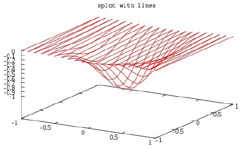
使用lines选项把每个点用线接连起来:
splot `data3d.dat` with lines notitle
也可以通过dgrid3d指定用网格来显示:
set dgrid3d 50,50
set hidden3d
replot
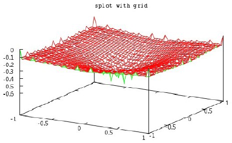
上面图里的网络与文件中的数值不同,原因是网格默认会对Z轴上的值做出平均。
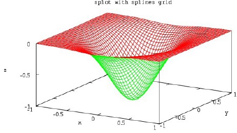
通过splines禁止自动平均:
set dgrid3d splines
set xlabel 'x'
set ylabel 'y'
set zlabel 'z'
set title 'splot with splines grid'
set ticslevel 0
set ztics -1, 0.5, 0
replot
极坐标模式
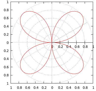
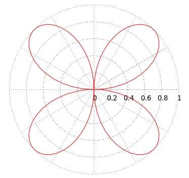
极坐标模式绘图
-
set polar指定极坐标模式 -
默诵变量为
t,默认取值范围是\(0\)~\(2\pi\) -
set size ration 1指定高宽比为1
set polar
set xrange [-1:1]
set yrange [-1:1]
set grid polar
set size ratio 1
set xtics 0.2
set ytics 0.2
plot sin(2*t) notitle
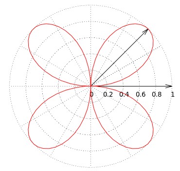
如果想要把方的线都去掉,可以做以下调整:
- 如果要去掉边框,可以设置边框线为宽为0。
- 把x轴和y轴的标注都改为白色的,这样就看不见了。
set border linewidth 0
set xtics textcolor rgbcolor 'white'
set ytics textcolor rgbcolor 'white'
replot
还可以加上两个箭头:
set arrow from 0,0 to 1,0
set arrow from 0,0 to 0.707,0.707
replot
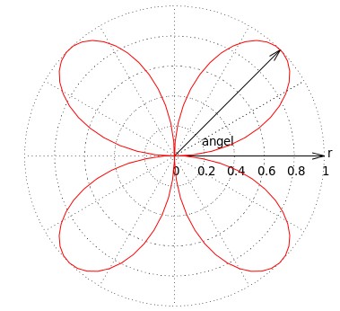
要指定的坐标上给加上注解「r」和「angel」:
set label 'angel' at 0.18,0.1
set label 'r'     at 1.02,0.02
replot
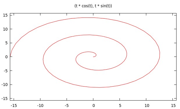
参数方程作图
-
set parametric指定为参数方程。 -
set size ration 1指定高宽比为1 -
曲线作图默认变量
t,默认范围\([-5, 5]\) -
曲面作图默认变量
u和t,默认范围\([-10, 10]\)
set parametric
set trange [0       : 5 * pi]
set xrange [-5 * pi : 5 * pi]
set yrange [-5 * pi : 5 * pi]
set size ration 1
set title '(t * cos(t), t * sin(t))'
plot t * cos(t), t * sin(t) notitle
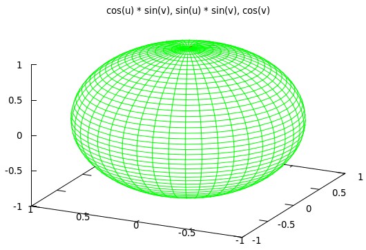
set parametric
set urange [0:2*pi]
set vrange [0:pi]
set xrange [-1:1]
set yrange [-1:1]
set zrange [-1:1]
set isosamples 45,45
set hidden3d
set ticslevel 0             # 平移z轴
set view 60, 30, 1, 1.5     # 视角
set title 'cos(u) * sin(v), sin(u) * sin(v), cos(v)'
splot cos(u) * sin(v), sin(u) * sin(v), cos(v) notitle