OpenCV 图像变形

基本的矩阵操作

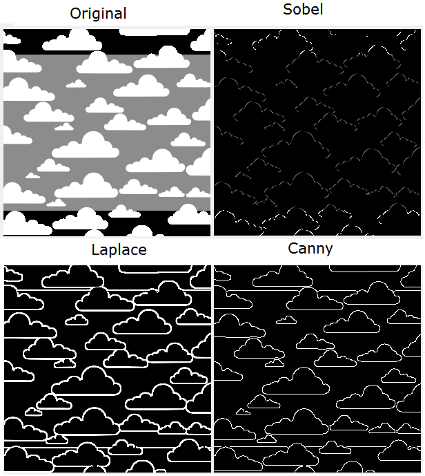
梯度和索贝尔导数

Sobel kernel matrix:

\[ G_x = \begin{bmatrix} -1 & 0 & +1 \\ -2 & 0 & 2 \\ -1 & 0 & 1 \\ \end{bmatrix} \times T_x \]

Imgproc中的Sobel函数：

public static void Sobel(Mat src, Mat dst, int ddepth, int dx, int dy)

拉普拉斯变换和Canny变换

主要用来二值化图片上的变化。

Laplace transform:

\[ Laplace(f) = \frac{\partial{}^2f}{\partial{}x^2} + \frac{\partial{}^2f}{\partial{}y^2} \]

默认的3x3矩阵是这个样子：

\[ \begin{bmatrix} 0 & 1 & 0 \\ 1 & -4 & 1 \\ 0 & 1 & 0 \\ \end{bmatrix} \]

Imgproc中的Laplacian方法签名：

public static void Laplacian(Mat source, Mat destination, int ddepth)

Imgproc中的Canny方法签名：

public static void Canny(Mat image, Mat edges, double threshold1, 
		double threshold2, int apertureSize, boolean L2gradient)

用霍夫变换找到线与圆

Hough transforms

HoughLines(Mat image, Mat lines, double rho, double theta, int threshold)

HoughLinesP(Mat image, Mat lines, double rho, double theta, int threshold)

Mat canny = new Mat();
// Imgproc.Canny(originalImage, canny, 10, 50, aperture, false);
Imgproc.cvtColor(originalImage, canny, Imgproc.COLOR_BGR2GRAY);
Imgproc.blur(canny, canny, new Size(3, 3));
image = originalImage.clone();
Mat lines = new Mat();
Imgproc.HoughLines(canny, lines, 1, Math.PI/180, lowThreshold);

几何变形

常用的几何变形有：拉伸、收缩、折叠、旋转。 指定8个点（就是两人个平行四边开），指定拉伸前和拉伸后的变形关系：

import org.opencv.core.MatOfPoint2f;

public static Mat getPerspectiveTransform(Mat src, Mat dst)

public static void warpPerspective(Mat src, Mat dst, Mat M, Size dsize)

有的时候点的x与y是浮点数，所以getPerspectiveTransform() 参数的矩阵类型为org.opencv.core.MatOfPoint2f。

例子：

/* 8个点 */
val srcPoints = Array(
		new Point(296.0,  40.0), 
		new Point(577.0, 223.0), 
		new Point(296.0, 387.0), 
		new Point(577.0, 362.0))

val dstPoints = Array(
		new Point(0.0,  0.0), 
		new Point(oriImage.width - 1, 0), 
		new Point(0.0, oriImage.height - 1), 
		new Point(oriImage.width - 1, oriImage.height - 1))

/* 组成两人个开行四边形 */
val srcTri = new MatOfPoint2f(srcPoints(0), srcPoints(1), srcPoints(2), srcPoints(3));
val dstTri = new MatOfPoint2f(dstPoints(0), dstPoints(1), dstPoints(2), dstPoints(3));

/* 变形 */
val warpMat = Imgproc.getPerspectiveTransform(srcTri, dstTri);
val destImage = new Mat();
Imgproc.warpPerspective(oriImage, destImage, warpMat, oriImage.size());

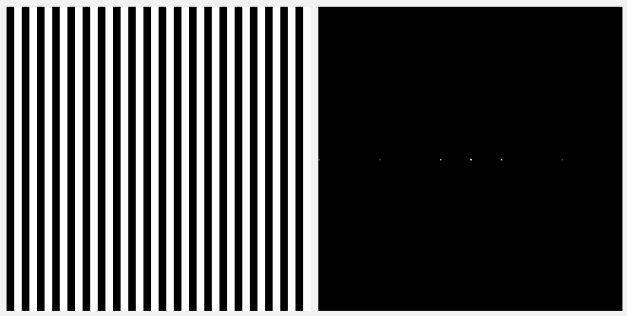
傅利叶变换

DFT：

\[ F(k, l) = \sum_{i=0}^{N-1}\sum_{i=0}^{N-1}f(i,j)e^{-i2\pi{\big(\frac{ki}{N}+\frac{lj}{N}\big)}} \]

The following code shows you how to make room to apply the DFT. Remember, from the preceding screenshot, that the result of a DFT is complex. Besides, we need them stored as floating point values. This way, we first convert our 3-channel image to gray and then to a float. After this, we put the converted image and an empty Mat object into a list of mats, combining them into a single Mat object through the use of the Core.merge function, shown as follows:

val gray = new Mat()
Imgproc.cvtColor(oriImage, gray, Imgproc.COLOR_RGB2GRAY)

// 转为浮点数，进行傅利叶变换
val floatGray = new Mat() 
gray.convertTo(floatGray, CvType.CV_32FC1)

val matList = new java.util.ArrayList[Mat]()
matList.add(floatGray)
val zeroMat = Mat.zeros(floatGray.size(), CvType.CV_32F)
matList.add(zeroMat)
val complexImage = new Mat()
Core.merge(matList, complexImage)

Now, it's easy to apply an in-place Discrete Fourier Transform:

Core.dft(complexImage, complexImage)

have to obtain its magnitude. In order to get it, we will use the standard way that we learned in school, which is getting the square root of the sum of the squares of the real and complex parts of numbers.

Again, OpenCV has a function for this, which is Core.magnitude, whose signature is magnitude(Mat x, Mat y, Mat magnitude), as shown in the following code.

Before using Core.magnitude, just pay attention to the process of unpacking a DFT in the splitted mats using Core.split:

val splitted = new java.util.ArrayList[Mat]()
Core.split(complexImage, splitted)
val magnitude = new Mat()
Core.magnitude(splitted.get(0), splitted.get(1), magnitude)

Since the values can be in different orders of magnitude, it is important to get the values in a logarithmic scale. Before doing this, it is important to add 1 to all the values in the matrix just to make sure we won't get negative values when applying the log function. Besides this, there's already an OpenCV function to deal with logarithms, which is Core.log:

Core.add(Mat.ones(magnitude.size(), CvType.CV_32F), magnitude, magnitude)
Core.log(magnitude, magnitude)

Now, it is time to shift the image to the center, so that it's easier to analyze its spectrum. The code to do this is simple and goes like this:

val cx = magnitude.cols() / 2
val cy = magnitude.rows() / 2

val q0 = new Mat(magnitude, new Rect( 0,  0, cx, cy)) // Top-Left - Create a ROI per quadrant
val q1 = new Mat(magnitude, new Rect(cx,  0, cx, cy)) // Top-Right
val q2 = new Mat(magnitude, new Rect( 0, cy, cx, cy)) // Bottom-Left
val q3 = new Mat(magnitude, new Rect(cx, cy, cx, cy)) // Bottom-Right

val tmp = new Mat()  // swap quadrants (Top-Left with Bottom-Right)
q0.copyTo(tmp)
q3.copyTo(q0)
tmp.copyTo(q3)

q1.copyTo(tmp)       // swap quadrant (Top-Right with Bottom-Left)
q2.copyTo(q1)
tmp.copyTo(q2)

As a last step, it's important to normalize the image, so that it can be seen in a better way. Before we normalize it, it should be converted to CV_8UC1:

magnitude.convertTo(magnitude, CvType.CV_8UC1)
Core.normalize(magnitude, magnitude, 0, 255, Core.NORM_MINMAX, CvType.CV_8UC1)

When using the DFT, it's often enough to calculate only half of the DFT when you deal with real-valued data, as is the case with images. This way, an analog concept called the Discrete Cosine Transform can be used. In case you want it, it can be invoked through Core.dct.

Integral Images

Some face recognition algorithms, such as OpenCV's face detection algorithm make heavy use of features like the ones shown in the following image:

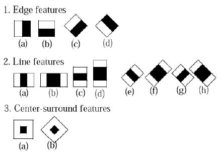
These are the so-called Haar-like features and they are calculated as the sum of pixels in the white area minus the sum of pixels in the black area. You might find this type of a feature kind of odd, but when training it for face detection, it can be built to be an extremely powerful classifier using only two of these features, as depicted in the following image:

In fact, a classifier that uses only the two preceding features can be adjusted to detect 100 percent of a given face training database with only 40 percent of false positives. Taking out the sum of all pixels in an image as well as calculating the sum of each area can be a long process. However, this process must be tested for each frame in a given input image, hence calculating these features fast is a requirement that we need to fulfill.

First, let's define an integral image sum as the following expression:

\[ sum(X,Y) = \sum_{x\lt{}X}\sum_{y\lt{}Y}image(x,y) \]

For instance, if the following matrix represents our image:

\[ A = \begin{bmatrix} 0 & 2 & 4 \\ 6 & 8 & 10 \\ 12 & 14 & 16 \\ \end{bmatrix} \]

An integral image would be like the following:

\[ Sum(A) = \begin{bmatrix} 0 & 0 & 0 & 0 \\ 0 & 0 & 2 & 6 \\ 0 & 6 & 16 & 30 \\ 0 & 18 & 42 & 72 \\ \end{bmatrix} \]

The trick here follows from the following property:

\[ \sum_{x1\le{}x\le{}x2}\sum_{y1\le{}y\le{}y2}image(x,y) = sum(x2,y2) - sum(x1-1,y2) - sum(x2, y1-1) + sum(x1-1, y1-1) \]

This means that in order to find the sum of a given rectangle bounded by the points (x1,y1), (x2,y1), (x2,y2), and (x1,y2), you just need to use the integral image at the point (x2,y2), but you also need to subtract the points (x1-1, y2) from (x2,y1-1). Also, since the integral image at (x1-1, y1-1) has been subtracted twice, we just need to add it once.

The following code will generate the preceding matrix and make use of Imgproc.integral to create the integral images:

Mat image = new Mat(3,3 ,CvType.CV_8UC1);
Mat sum = new Mat();
byte[] buffer = {0,2,4,6,8,10,12,14,16};
image.put(0,0,buffer);
System.out.println(image.dump());
Imgproc.integral(image, sum);
System.out.println(sum.dump());

The output of this program is like the one shown in the preceding matrices for A and Sum A.

It is important to verify that the output is a 4 x 4 matrix because of the initial row and column of zeroes, which are used to make the computation efficient.

距离变换

突出图像上的像素与黑色背景的距离，用来突出显示图像的拓扑骨架：

Imgproc.threshold(image, image, 100, 255, Imgproc.THRESH_BINARY);
Imgproc.distanceTransform(image, image, Imgproc.CV_DIST_L2, 3);
image.convertTo(image, CvType.CV_8UC1);
Core.multiply(image, new Scalar(20), image);

一般在应用中会额外加上Canny过滤操作突出图像的边缘：

Imgproc.Canny(oriImage, image, 220, 255, 3, false);
Imgproc.threshold(image, image, 100, 255, Imgproc.THRESH_BINARY_INV);
Imgproc.distanceTransform(image, image, Imgproc.CV_DIST_L2, 3);
image.convertTo(image, CvType.CV_8UC1);
Core.multiply(image, new Scalar(20), image);

投影平衡

投影用来分析图片。当图片的明暗区间非常小的时候，会不容易分辨细节。

下面的图片加大了明暗对比，所以细节看起来更加明显，但是因为是后期拉大的范围， 可以看到过渡不自然，尤其是云上的过渡有明显的断层：

// 把彩色图转为灰度
val grayImage = oriImage.clone()
Imgproc.cvtColor(oriImage, grayImage, Imgproc.COLOR_RGB2GRAY);

// 再按灰度图为基础拉大明暗区域
val image = new Mat() 
Imgproc.equalizeHist(grayImage, image);