ch01 构造过程抽象 part02
过程与它们所产生的计算
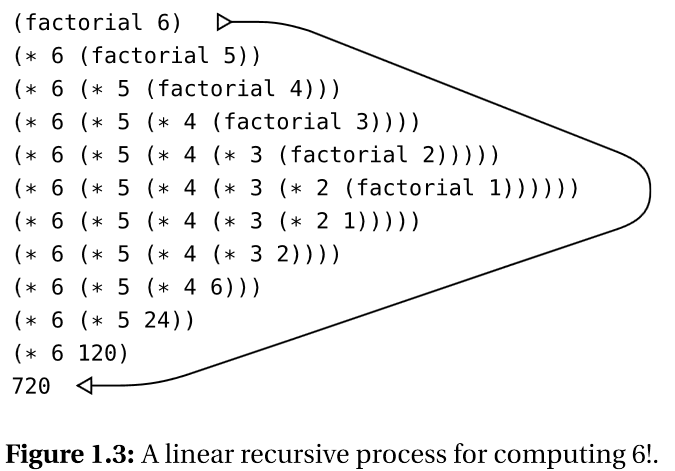
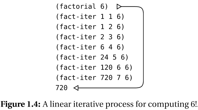
线性的递归与迭代
以典型的阶乘\(n!\)为例。
\[ \begin{equation} n! = n \cdot (n-1) \cdot (n - 2) \cdots 3 \cdot 2 \cdot 1 \end{equation} \]阶乘的计算过程可能用「递归」和「迭代」两种方式来描述(注意这里的「递归」和 「迭代」都是指计算展开方式,而不是程序语法上的)。
线性递归过程
\[ \begin{equation} \begin{split} n! &= n \cdot (n-1) \cdot (n - 2) \cdots 3 \cdot 2 \cdot 1 \\ &= n \cdot [ (n-1) \cdot (n - 2) \cdots 3 \cdot 2 \cdot 1 ] \\ &= n \cdot (n-1)! \end{split} \end{equation} \]
(define (factorial n)
  (if (= n 1)
      1
      (* n (factorial (- n 1)))))    ; <- 对自己的递归调用不是最后一个动作,
                                     ;    所以要保留n
- 递归计算过程(recursive process):计算过程可描述为由一个推迟(deferred operations)执行的运算链条。
- 线性递归过程(linear recursive process):需要维护操作的轨迹信息,这个长度 随着\(n\)的值线性增长
- 在递归过程中,解释器维护的操作轨迹就是程序执行到了第几步。
线性迭代过程
线性迭代(linear iterative process)时要额外记录两个数值:
- 计数(connter)
- 乘积(product)
(define (factorial n)
  (fact-iter 1 1 n))

(define (fact-iter product counter max-count)
  (if (> counter max-count)
      product
      (fact-iter (* counter product)
                 (+ counter 1)
                 max-count)))
- 迭代的过程中没有展开与收缩过程。
- 迭代过程中计算状态全由变量来保存的,可以直接通过设置变量的值来恢复到执行中的 第n步。
语法递归与计算递归的区别
- 语法形式上的:递归「过程」,是指在语法上一个过程(直接或间接地)调用该过程本身。
- 计算过程上的:递归「计算」,是指计算过程的展开方式。
练习 1.9
方法inc和dec分别实现把参数加1或减1。下面是分别用这两个方法实现的正整数
相加语法:
(define (+ a b)
  (if (= a 0)
      b
      (inc (+ (dec a) b))))

(define (+ a b)
  (if (= a 0)
      b
      (+ (dec a) (inc b))))
用代换模型展示这两个过程在求值(+ 4 5)的计算过程,并指出这些过程是递归还是
迭代的?
以下是第一个+函数的定义(为了和内置的+区分开来,我们将函数改名为plus):
(load "9-inc.scm")
(load "9-dec.scm")

(define (plus a b)
    (if (= a 0)
        b
        (inc (plus (dec a) b))))
对(plus 3 5)进行求值,表达式的展开过程为:
(plus 3 5)
(inc (plus 2 5))
(inc (inc (plus 1 5)))
(inc (inc (inc (plus 0 5))))
(inc (inc (inc 5)))
(inc (inc 6))
(inc 7)
8
从计算过程中可以很明显地看到伸展和收缩两个阶段,且伸展阶段所需的额外存储量和
计算所需的步数都正比于参数a,说明这是一个线性递归计算过程。
另一个+函数
;;; 9-another-plus.scm

(load "9-inc.scm")
(load "9-dec.scm")

(define (plus a b)
    (if (= a 0)
        b
        (plus (dec a) (inc b))))
对(plus 3 5)进行求值,表达式的展开过程为:
(plus 3 5)
(plus 2 6)
(plus 1 7)
(plus 0 8)
8
从计算过程中可以看到,这个版本的plus函数只使用常量存储大小,且计算所需的步骤
正比于参数a,说明这是一个线性迭代计算过程。
使用 trace 追踪调用
我们还可以配合trace函数,通过在解释器里面追踪两个plus函数的不同定义来考察
它们所使用的计算模式。
首先来追踪第一个plus函数:
1 ]=> (load "9-plus.scm")

;Loading "9-plus.scm"...
;  Loading "9-inc.scm"... done
;  Loading "9-dec.scm"... done
;... done
;Value: plus

1 ]=> (trace plus)

;Unspecified return value

1 ]=> (plus 3 5)

[Entering #[compound-procedure 11 plus]
    Args: 3
          5]
[Entering #[compound-procedure 11 plus]
    Args: 2
          5]
[Entering #[compound-procedure 11 plus]
    Args: 1
          5]
[Entering #[compound-procedure 11 plus]
    Args: 0
          5]
[5
    <== #[compound-procedure 11 plus]
    Args: 0
          5]
[6
    <== #[compound-procedure 11 plus]
    Args: 1
          5]
[7
    <== #[compound-procedure 11 plus]
    Args: 2
          5]
[8
    <== #[compound-procedure 11 plus]
    Args: 3
          5]
;Value: 8
从trace打印的结果来看,plus的参数b在伸展和收缩阶段都一直是5,最后的结果
是根据inc函数递归计算而来的。
然后来看看第二个 plus :
1 ]=> (load "9-another-plus.scm")

;Loading "9-another-plus.scm"...
;  Loading "9-inc.scm"... done
;  Loading "9-dec.scm"... done
;... done
;Value: plus

1 ]=> (trace plus)

;Unspecified return value

1 ]=> (plus 3 5)

[Entering #[compound-procedure 11 plus]
    Args: 3
          5]
[Entering #[compound-procedure 11 plus]
    Args: 2
          6]
[Entering #[compound-procedure 11 plus]
    Args: 1
          7]
[Entering #[compound-procedure 11 plus]
    Args: 0
          8]
[8
    <== #[compound-procedure 11 plus]
    Args: 0
          8]
[8
    <== #[compound-procedure 11 plus]
    Args: 1
          7]
[8
    <== #[compound-procedure 11 plus]
    Args: 2
          6]
[8
    <== #[compound-procedure 11 plus]
    Args: 3
          5]
;Value: 8
从trace的结果可以看出,第二个plus的计算过程并没有伸展和收缩阶段,它通过不断
更新a和b两个参数的值来完成计算。
练习 1.10
下面是一个经典的数学函数叫Ackermann函数:
(define (A x y)
  (cond ((= y 0) 0)
        ((= x 0) (* 2 y))
        ((= y 1) 2)
        (else (A (- x 1)
                 (A x (- y 1))))))
然后使用 A 函数对题目给定的几个表达式求值:
1 ]=> (load "10-ackermann.scm")
;Loading "10-ackermann.scm"... done
;Value: a

1 ]=> (A 1 10) ;Value: 1024

1 ]=> (A 2 4) ;Value: 65536

1 ]=> (A 3 3) ;Value: 65536
对于下面的过程,f、g、h对给定数值n所计算的函数的数学定义。例如:
(k n)计算的是\(5n^2\)。
(define (f n) (A 0 n))

(define (g n) (A 1 n))

(define (h n) (A 2 n))

(define (k n) (* 5 n n))
接着,我们通过给定一些连续的n,来观察题目给出的几个函数,从而确定它们的
数学定义。
首先是(define (f n) (A 0 n)):
| n | 0 | 1 | 2 | 3 | 4 | 5 | 6 | 7 | ... | |
|---|---|---|---|---|---|---|---|---|---|---|
| 值 | 0 | 2 | 4 | 6 | 8 | 10 | 12 | 14 | ... |
可以看出,函数f计算的应该是\(2 \times n\)。
然后是(define (g n) (A 1 n)):
| n | 0 | 1 | 2 | 3 | 4 | 5 | 6 | 7 | ... |
|---|---|---|---|---|---|---|---|---|---|
| 值 | 0 | 2 | 4 | 8 | 16 | 32 | 64 | 128 | ... |
可以看出,函数g计算的应该是\(2^n\)。
最后是(define (h n) (A 2 n)):
| n | 0 | 1 | 2 | 3 | 4 | 5 | 6 | 7 | ... |
|---|---|---|---|---|---|---|---|---|---|
| 值 | 0 | 2 | 4 | 16 | 65536 | ... | ... | ... | ... |
当n超过4之后,再调用函数h就会出现超出解释器最大递归深度的现象,从仅有的
几个计算结果来看,猜测函数h计算的应该是连续求n次二次幂,也即是:
树形递归
斐波哪契数列的定义:
\[ Fib(n)=\begin{cases} \begin{equation} \begin{split} & 0 & \text{当:} n=0 \\ & 1 & \text{当:} n=1 \\ & Fib(n-1) + Fib(n-2) & \text{其他情况} \end{split} \end{equation} \end{cases} \]
(define (fib n)
  (cond ((= n 0) 0)
        ((= n 1) 1)
        (else (+ (fib (- n 1))
                 (fib (- n 2))))))
树形递归造成大量重复计算
这样的展开是树形的:
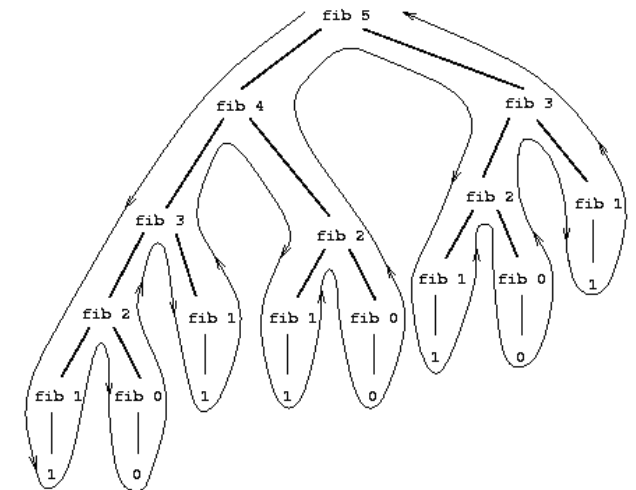
问题在于(fib 3)重复做了两次,(fib 0)和(fib 1)的次数正好是\(Fib(n + 1)\)。
Fib(n)的值就是最接近\(\phi^n / \sqrt{5}\)的整数。
其中\(\phi\)为黄金分割:
\[ \phi = \frac{1 + \sqrt{5}}{2} \approx 1.6180 \]它满足:
\[ \phi^2 = \phi + 1 \]- Fib方法的步骤随输入指数性增长
- 空间需求随输入线性地增加
用替换方式取代树形递归
设计一个迭代的计算过程,基本思想是用一对整数\(a\)和\(b\),将它们初始化为\(Fib(1) = 1\) 和\(Rib(0) = 0\),然后反复使用下面的规则:
\[ \begin{equation} \begin{split} a & \gets a + b \\ b & \gets a \end{split} \end{equation} \]这样在\(n\)次应用这些变换以后,\(a\)与\(b\)分别等于\(Fib(n + 1)\)与\(Fib(n)\)。程序为:
(define (fib n)
  (fib-iter 1 0 n))

(define (fib-iter a b count)
  (if (= count 0)
      b
      (fib-iter (+ a b) a (- count 1))))
这个方法性能相对于\(n\)为线性的,要好很多。
虽然树形迭代性能不好,但是也有它的用处。对于非数值操作而是层次结构数据时就
很有用。而且在上个fib程序中虽然树形的性能不好,但易于理解。
实例:换零钱方式的统计
100美分等于1美元,对于1美分、5美分、10美分、25美分、50美分这几种面值的硬币。 1美元有多少种换法?
对于任意数量的现金,能写出程序计算出所有换零钱的方式么?
先把硬币种类排序,总数为\(a\)的现金换成\(n\)种硬币的方式数等于:
- Step 1:\(a\)除第一种硬币外其他硬币的不同方式。
- Step 2:加上\(a - d\)换成所有种类硬币不同方式数目(\(d\)是第一种硬币的币值)。
上面相当于把可能性分成了两组:
- 没有用第一种面额
- 用了第一种面额以后的所有可能性
算法:
\[ \text{换零钱的方式}=\begin{cases} \begin{equation} \begin{split} & 1 \quad & \text{当:} a = 0 \\ & 0 \quad & \text{当:} a \lt 0 \\ & 0 \quad & \text{当:} n = 0 \end{split} \end{equation} \end{cases} \]树形递归:
;; 各个编号对应的面值
(define (first-denomination kinds-of-coins)
  (cond ((= kinds-of-coins 1) 1)
        ((= kinds-of-coins 2) 5)
        ((= kinds-of-coins 3) 10)
        ((= kinds-of-coins 4) 25)
        ((= kinds-of-coins 5) 50)))

;; 根据金额与一种具体的面值,算出有多少种分法
(define (cc amount kinds-of-coins)
  (cond ((= amount 0) 1)
        ((or (< amount 0) (= kinds-of-coins 0)) 0)
        (else (+ (cc amount
                     (- kinds-of-coins 1))
                 (cc (- amount
                        (first-denomination kinds-of-coins))
                     kinds-of-coins)))))

;; 根据金额算出有多少种分法
(define (count-change amount)
  (cc amount 5))

;: (count-change 100)          ; Value is 292
思考:如何把这个树形递归转为迭代递归?
习题 1.11
函数\(f\)的定义为:
\[ f(n) = \begin{cases} \begin{equation} \begin{split} & n & \text{当:} n \lt 3 \\ & f(n - 1) + 2f(n - 2) + 3f(n - 3) \quad & \text{当:} n \ge 3 \end{split} \end{equation} \end{cases} \]写出递归计算过程与迭代计算过程。
;;; 11-rec.scm

(define (f n)
    (if (< n 3)
        n
        (+ (f (- n 1))
           (* 2 (f (- n 2)))
           (* 3 (f (- n 3))))))
测试这个递归版的 f :
(load "11-rec.scm")

(f 1) ;Value: 1
(f 3) ;Value: 4
(f 4) ;Value: 11
迭代版本
要写出函数 f 的迭代版本,关键是在于看清初始条件和之后的计算进展之间的关系, 就像书本 25-26 页中,将斐波那契函数从递归改成迭代那样。
\[ \begin{equation} \begin{split} f(0) &=0 \\ f(1) &=1 \\ f(2) &=2 \\ f(3) &=f(2)+2f(1)+3f(0) \\ f(4) &=f(3)+2f(2)+3f(1) \\ f(5) &=f(4)+2f(3)+3f(2) \\ … \end{split} \end{equation} \]可以看出,当\(n \gt 3\)时,所有函数\(f\)的计算结果都可以用比当前\(n\)更小的三个 \(f\)调用计算出来。
迭代版的函数定义如下:
它使用i作为渐进下标,n作为最大下标,a、b和c三个变量分别代表函数调用
f(i+2)、f(i+1)和f(i),从f(0)开始,一步步计算出f(n):
;;; 11-iter.scm

(define (f n)
    (f-iter 2 1 0 0 n))

(define (f-iter a b c i n)
    (if (= i n)
        c
        (f-iter (+ a (* 2 b) (* 3 c))   ; new a
                a                       ; new b
                b                       ; new c
                (+ i 1)                 ; new i
                n)))                    ; still n
测试这个迭代版的函数:
(load "11-iter.scm")

(f 1) ;Value: 1
(f 3) ;Value: 4
(f 4) ;Value: 11
改进:其实不用i,直接用(- n 1)来计数就可以了:
(define (f n) (f-iter 0 1 2 n))

(define (f-iter x y z n)
	(if (= n 0)
		x
		(f-iter y z (+ z (* 2 y) (* 3 x)) (- n 1))))
练习 1.12
帕斯卡三角:
    1
   1 1
  1 2 1
 1 3 3 1
1 4 6 4 1
...
边上都是1,里面的数字等于左上右上两个加起来。其中的第n行就是\((x + y)^n\)的
展开式的系数。
写出递归计算过程。
Warning:这道练习的翻译有误,原文是「...Write a procedure that computes elements of Pascal’s triangle by means of a recursive process.」,译文只翻译了 「。。。它采用递归计算过程计算出帕斯卡三角形。」,这里应该是「帕斯卡三角形的 各个元素」才对。
使用示例图可以更直观地看出帕斯卡三角形的各个元素之间的关系:
row:
0        1
1       1 1
2      1 2 1
3     1 3 3 1
4    1 4 6 4 1
5   . . . . . .
col: 0 1 2 3 4
如果使用pascal(row, col)代表第row行和第col列上的元素的值,可以得出一些
性质:
-
每个
pascal(row, col)由pascal(row-1, col-1)(左上边的元素)和pascal(row-1, col)(右上边的元素)组成。 -
当
col等于0(最左边元素),或者row等于col(最右边元素)时,pascal(row, col)等于1。
比如说,当row = 3,col = 1时,pascal(row,col)的值为3,而这个值又是根据
pascal(3-1, 1-1) = 1和pascal(3-1, 1) = 2计算出来的。
综合以上的两个性质,就可以写出递归版本的 pascal 函数了:
;;; 12-rec-pascal.scm

(define (pascal row col)
    (cond ((> col row)
            (error "unvalid col value"))
          ((or (= col 0) (= row col))
            1)
          (else (+ (pascal (- row 1) (- col 1))
                   (pascal (- row 1) col)))))
测试一下这个 pascal 函数:
(load "12-rec-pascal.scm")

(pascal 4 0) ;Value: 1
(pascal 4 4) ;Value: 1
(pascal 4 2) ;Value: 6
迭代版本的 pascal 函数
前面给出的递归版本pascal函数的效率并不好,首先,因为它使用的是递归计算方式,
所以它的递归深度受限于解释器所允许的最大递归深度。
其次,递归版本pascal函数计算值根据的是公式:
这个公式带有重复计算,并且复杂度也很高,因此,前面给出的pascal函数只能用于
row和col都非常小的情况。
要改进这一状况,可以使用帕斯卡三角形的另一个公式来计算帕斯卡三角形的元素:
\[ {row \choose col} = \frac{row!}{col! \cdot (row-col)!} \]
其中row!表示row的阶乘(factorial)。
阶乘可以利用书本 22 页的factorial函数(迭代版)来计算:
;;; p22-iter-factorial.scm

(define (factorial n)
    (fact-iter 1 1 n))

(define (fact-iter product counter max-count)
    (if (> counter max-count)
        product
        (fact-iter (* counter product)
                   (+ counter 1)
                   max-count)))
然后,使用factorial和给定的公式,给出迭代版本的pascal定义:
;;; 12-iter-pascal.scm

(load "p22-iter-factorial.scm")

(define (pascal row col)
    (/ (factorial row)
       (* (factorial col)
          (factorial (- row col)))))
迭代版的pascal函数消除了递归版pascal的重复计算,并且它是一个线性复杂度的
算法,因此,迭代版的pascal比起递归版的pascal要快不少,并且计算的值的大小
不受递归栈深度的控制:
(load "12-iter-pascal.scm")

(pascal 4 0)      ;Value: 1
(pascal 4 4)      ;Value: 1
(pascal 4 2)      ;Value: 6
(pascal 1024 256) ;Value: 346269144346889986395924831854035885865562696970381965629886488418277363006094610102022787857042680079787023567910689787903778413121916299434613646920250770005333708478791829291433521372230388837458830111329620101516314992938333258379799593534242588
最后一个测试尝试了对(pascal 1024 256)进行求值,计算结果是一个蛮大的数,如果
使用递归版的pascal函数的话,这种计算就要非常非常久了,但是迭代版本还是可以
很快地算出来。
See also
有很多不同的方式可以计算帕斯卡三角形的各个元素,可以参考维基百科的 Pascal’s triangle 页面、 Binomial coefficient 页面,或者任何一本组合数学方面的书籍。
练习 1.13
证明Fib(n)的值就是最接近\(\phi^n / \sqrt{5}\)的整数。其中\(\phi\)为黄金分割:
提示:利用归纳法和斐波那契数的定义,证明:
\[ Fib(n) = \frac{\phi^n - \gamma^n}{\sqrt{5}} \]解答过程:
首先证明
\[ Fib(n) = \frac{\phi^{n}-\psi^{n}}{\sqrt{5}} \]设
\[ Fib(n) = \frac{\phi^{n}-\psi^{n}}{\sqrt{5}} \]则
\(Fib(n+1)\)的推导:
\[ \begin{equation} \begin{split} Fib(n+1) & = \frac{\phi^{n+1}-\psi^{n+1}}{\sqrt{5}} \\ & = \frac{\phi^{n} \cdot \phi - \psi^{n} \cdot \psi}{\sqrt{5}} \\ & = \frac{\phi^{n} \cdot \frac{1+\sqrt{5}}{2} - \psi^{n} \cdot \frac{1-\sqrt{5}}{2}}{\sqrt{5}} \\ & = \frac{1}{2} \cdot \left( \frac{\phi^{n} - \psi^{n}}{\sqrt{5}} + \frac{\sqrt{5} \cdot \left( \phi^{n} + \psi^{n} \right) }{\sqrt{5}} \right) \\ & = \frac{1}{2} \cdot Fib(n) + \frac{\phi^{n} + \psi^{n}}{2} \end{split} \end{equation} \]\(Fib(n+2)\)的推导:
\[ \begin{equation} \begin{split} Fib(n+2) & = \frac{\phi^{n+2}-\psi^{n+2}}{\sqrt{5}} \\ & = \frac{\phi^{n} \cdot \phi^{2} - \psi^{n} \cdot \psi^{2}}{\sqrt{5}} \\ & = \frac{\phi^{n} \cdot (\frac{1+\sqrt{5}}{2})^{2} - \psi^{n} \cdot (\frac{1-\sqrt{5}}{2})^{2}}{\sqrt{5}} \\ & = \frac{1}{2} \cdot \left( \frac{3 \cdot (\phi^{n} - \psi^{n})}{\sqrt{5}} + \frac{\sqrt{5} \cdot (\phi^{n} + \psi^{n}) }{\sqrt{5}} \right) \\ & = \frac{3}{2} \cdot Fib(n) + \frac{\phi^{n} + \psi^{n}}{2} \\ \end{split} \end{equation} \]可证
\[ Fib(n+2) = Fib(n+1) + Fib(n) \]又
\[ \frac{\phi^{0}-\psi^{0}}{\sqrt{5}} = 0 = Fib(0) \] \[ \frac{\phi^{1}-\psi^{1}}{\sqrt{5}} = 1 = Fib(1) \]由此可知以下等式成立:
\[ Fib(n) = \frac{\phi^{n}-\psi^{n}}{\sqrt{5}} \]于是\(Fib(n)\)可以拆成两数之差的形式
\[ Fib(n) = \frac{\phi^{n}-\psi^{n}}{\sqrt{5}} = \frac{\phi^{n}}{\sqrt{5}}-\frac{\psi^{n}}{\sqrt{5}} \]而
\[ \frac{1}{\sqrt{5}} \lt \frac{1}{2} \] \[ |\psi| = |\frac{1-\sqrt{5}}{2}| \lt 1 \]故
\[ |\frac{\psi^{n}}{\sqrt{5}}| \lt \frac{1}{2} \]即
\[ |Fib(n) - \frac{\phi^{n}}{\sqrt{5}}| \lt \frac{1}{2} \]故得证:\(Fib(n)\)是与
\[ \frac{\phi^{n}}{\sqrt{5}} \]最接近的整数。
另一个解法。还可以用生成函数角法:
解递归方程:
\[ F_n = F_{n-1} + F_{n-2}, F_0 = 0, F_1 = 1 \]由生成函数:
\[ F(z) = \sum_{n \geq 0}F_nz^n \]满足:
\[ F(z) = zF(z) + z^2F(z) + z \]导出:
\[ F(z) = \frac{z}{1-z-z^2}= \frac{1}{\sqrt{5}}(\frac{1}{1-\phi z}-\frac{1}{1-\hat{\phi}z}) \]相加减:
\[ F_n = \frac{1}{\sqrt{5}}(\phi^n - \hat{\phi}^n) \]增长的阶
- \(n\):问题的规模
- \(R(n)\):处理规模为\(n\)的问题所需要的资源。
- \(f(n)\):\(n\)和\(R(n)\)的变化关系。
- \(\Theta(f(n))\):\(R(n)\)所具有增长的阶,读作\(f(n)\)的theta。
如果存在与\(n\)无关的整数\(k1\)和\(k2\),使得:
\[ k_1f(n) \leq R(n) \leq k_2f(n) \]在\(n\)无论多大时都成立(就是说对于足够大的\(n\),\(R(n)\)总在那两个之间)。就用 \(\Theta(f(n))\)表示\(R(n)\)增长的阶,记为:
\[ R(n) = \Theta(f(n)) \]- 对线性递归为例,步骤增长为\(\Theta(n)\),空间增长为\(\Theta(n)\);
- 对线性迭代为例,步骤增长为\(\Theta(n)\),空间增长为\(\Theta(1)\)(为常数)。
- 树形递归斐波那契,需要\(\Theta(\phi^n)\)步和\(\Theta(n)\)空间。这里的\(\phi\)为黄金 分割率。
这样的复杂度表示是很粗略的:因为\(1000n^2\)步和\(3n^2+10n+17\)都表示为\(\Theta(n^2)\) 。只有在规模增加一级时才表示出来。
练习 1.14
前面的换零钱程序count-change在换11美分成硬币时的计算过程的树,以及随金额增加
时增长的阶。
以下是(count-change 11)在运行时的展开过程
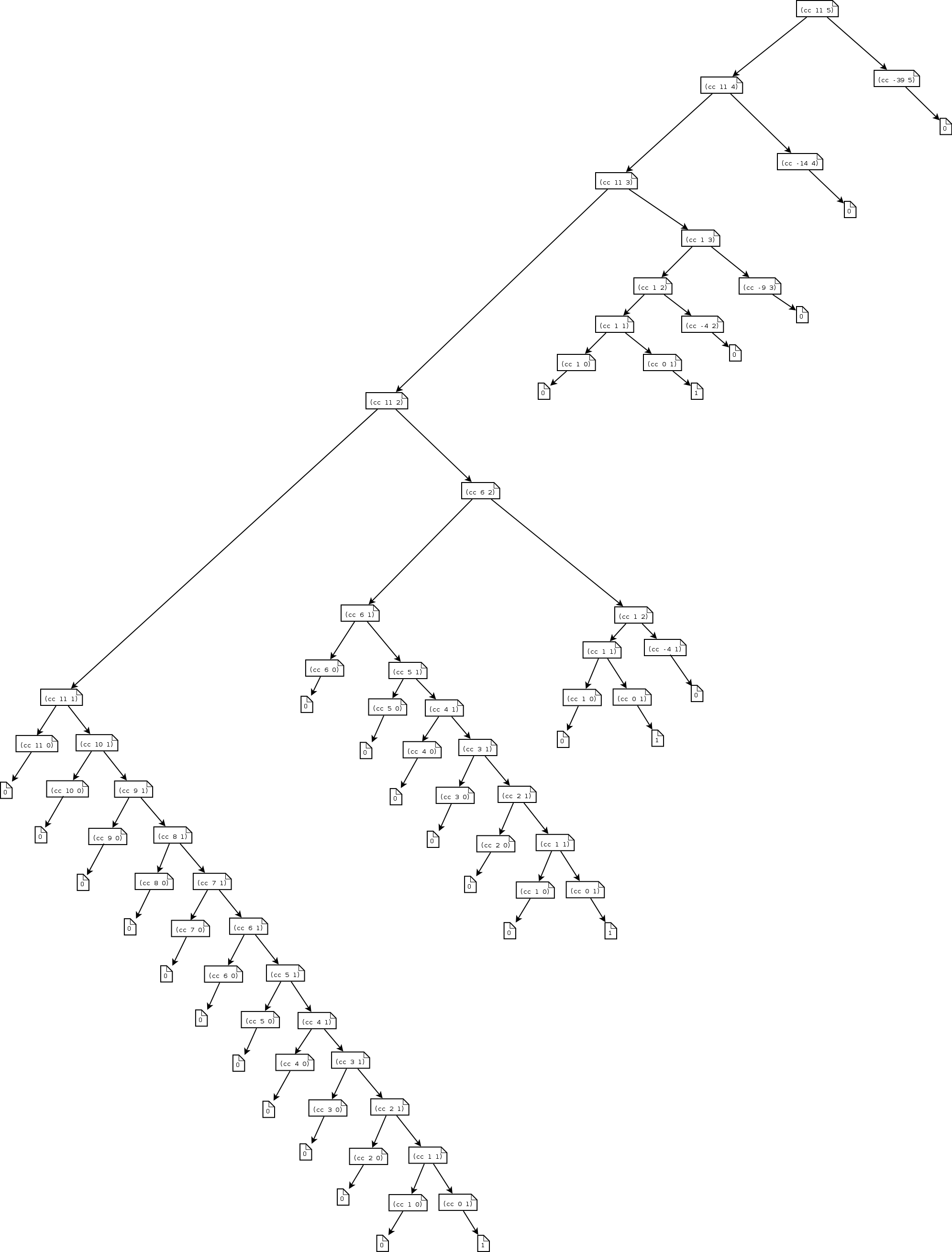
对于币种类\(m\)和金额\(n\),空间增长为\(\Theta(m + n)\),步骤增长为\(\Theta(n^m)\)。
练习 1.15
在角的弧度\(x\)足够小时,正弦值可以用\(\sin x \approx x\),而三角恒等式:
\[ \sin x = 3 \sin \frac{x}{3} - 4 \sin ^ 3 \frac{x}{3} \]可以减小\(\sin\)参数的大小(在这一题中,小于\(0.1\)的弧度认为是足够小的)。
这些想法用过程体现就是:
;;; 15.scm

(define (cube x) (* x x x))

(define (p x) (- (* 3 x) (* 4 (cube x))))

(define (sine angle)
    (if (not (> (abs angle) 0.1))
        angle
        (p (sine (/ angle 3.0)))))
在求值(sine 12.15)过程中,p将被调用多少次?
用 trace 追踪 p 的调用,计算它的运行次数:
1 ]=> (load "15.scm")

;Loading "15.scm"... done
;Value: sine

1 ]=> (trace-entry p)

;Unspecified return value

1 ]=> (sine 12.15)

[Entering #[compound-procedure 11 p]
    Args: 4.9999999999999996e-2]
[Entering #[compound-procedure 11 p]
    Args: .1495]
[Entering #[compound-procedure 11 p]
    Args: .4351345505]
[Entering #[compound-procedure 11 p]
    Args: .9758465331678772]
[Entering #[compound-procedure 11 p]
    Args: -.7895631144708228]
;Value: -.39980345741334

可以看到, p 共运行了 5 次。
在求值(sine a)时,使用的空间和步数增长的阶:
在求值(sine a)的时候,a每次都被除以3.0,而 sine 是一个递归程序,因此它的
时间和空间复杂度都是\(\Theta(\log a)\)。
如果以上预测是正确的话,那么每当 a 增大一倍(准确地说,是乘以因子 3), p 的运行 次数就会增加一次,以下是相应的测试:
1 ]=> (sine 10)                         ; 5 次 p 调用

[Entering #[compound-procedure 11 p]
    Args: .0411522633744856]
[Entering #[compound-procedure 11 p]
    Args: .12317802324595176]
[Entering #[compound-procedure 11 p]
    Args: .3620582351732319]
[Entering #[compound-procedure 11 p]
    Args: .8963314023464528]
[Entering #[compound-procedure 11 p]
    Args: -.19149217924571227]
;Value: -.5463890357524606

1 ]=> (sine 30)                         ; 6 次调用

[Entering #[compound-procedure 11 p]
    Args: .0411522633744856]
[Entering #[compound-procedure 11 p]
    Args: .12317802324595176]
[Entering #[compound-procedure 11 p]
    Args: .3620582351732319]
[Entering #[compound-procedure 11 p]
    Args: .8963314023464528]
[Entering #[compound-procedure 11 p]
    Args: -.19149217924571227]
[Entering #[compound-procedure 11 p]
    Args: -.5463890357524606]
;Value: -.9866890379958478

1 ]=> (sine 90)                         ; 7 次调用

[Entering #[compound-procedure 11 p]
    Args: .0411522633744856]
[Entering #[compound-procedure 11 p]
    Args: .12317802324595176]
[Entering #[compound-procedure 11 p]
    Args: .3620582351732319]
[Entering #[compound-procedure 11 p]
    Args: .8963314023464528]
[Entering #[compound-procedure 11 p]
    Args: -.19149217924571227]
[Entering #[compound-procedure 11 p]
    Args: -.5463890357524606]
[Entering #[compound-procedure 11 p]
    Args: -.9866890379958478]
;Value: .8823180886403317
求幂
对于\(b^n\)计算可以用递归的方法:
\[ \begin{equation} \begin{split} b^n &= b \times b^{n-1} \\ b^0 &= 1 \end{split} \end{equation} \]用过程表示为:
(define (expt b n)
	(if (= n 0)
		1
		(* b (expt b (- n 1)))))
这里的消耗是线性的,空间与步骤都是\(\Theta(n)\),优化为线性迭代:
(define (expt b n)
	(expt-iter b n 1))

(define (expt-iter b counter product)
	(if (= counter 0)
		product
		(expt-iter b
			(- counter 1)
			(* b product))))
这样空间缩小为\(\Theta(1)\)
可以用连续求平方方式进一步优化:
\[ b \times (b \times (b \times (b \times (b \times (b \times (b \times b)))))) \]相当于:
\[ \begin{equation} \begin{split} b^2 & = b \times b \\ b^4 & = b^2 \times b^2 \\ b^8 & = b^4 \times b^4 \end{split} \end{equation} \]进一步可以明白:
\[ \begin{equation} \begin{split} b^n &= (b^{n/2})^2 & \quad \quad \quad \text{如果$n$是偶数} \\ b^n &= b \times b^{n-1} & \quad \quad \quad \text{如果$n$是奇数} \end{split} \end{equation} \]写为过程就是:
(define (fast-expt b n)
	(cond ((= n 0) 1)
		((even? n) (square (fast-expt b (/ n 2))))
		(else (* b (fast-expt b (- n 1))))))
检查是否是偶数:
(define (even? n)
	(= (remainder n 2) 0))
现在来看,计算\(b^{2n}\)时只要比\(b^n\)多做算一次,所以增长为以2为底的n的对数, 表示为\(\Theta(log n)\)
练习 1.16
设计一个用迭代方式的求幂过程。(提示:利用关系\((b^{n/2})^2 = (b^2)^{n/2}\)
除了n和b以外再附加一个变量a,并定义好状态使得从一个状态到别一个状态时
\(a b^n\)不变。在计算过程开始是a为1,然后过程结束时以a值作为答案。一般来说,
定义一个不变量,要求它在状态之间保持不变,这一技术是思考迭代算法设计时的一种
非常有力的方法。)
程序:
;;; 16-fast-expt.scm

(define (fast-expt b n)
    (expt-iter b n 1))

(define (expt-iter b n a)
    (cond ((= n 0)
            a)
          ((even? n)
            (expt-iter (square b)
                       (/ n 2)
                       a))
          ((odd? n)
            (expt-iter b
                       (- n 1)
                       (* b a)))))
测试:
1 ]=> (load "16-fast-expt.scm")

;Loading "16-fast-expt.scm"... done
;Value: expt-iter

1 ]=> (fast-expt 2 0)

;Value: 1

1 ]=> (fast-expt 2 7)

;Value: 128

1 ]=> (fast-expt 2 10)

;Value: 1024
练习 1.17
本节中的幂算法是用反复乘法求幂。不用乘法只用加减法的版本如下:
(define (* a b)
	(if (= b 0)
		0
		(+ a (* a (- b 1)))))
如果现在再提供double和halve两个方法分别代表翻倍与减半,请设计一个fast-expt
的求乘积过程,优化操作步骤为对数增长。
首先写出double和halve两个辅助函数,其中double求出一个数的两倍,而halve
则将一个数除以2:
;;; 17-double-and-halve.scm

(define (double n)
    (+ n n))

(define (halve n)
    (/ n 2))
然后利用类似书本30页的fast-expt的技术,写出使用对数步数求乘积的函数(为了和
内置的*函数区分开,函数使用multi作为名字):
;;; 17-multi.scm

(load "17-double-and-halve.scm")

(define (multi a b)
    (cond ((= b 0)
            0)
          ((even? b)
            (double (multi a (halve b))))
          ((odd? b)
            (+ a (multi a (- b 1))))))
测试 double 和 halve :
1 ]=> (load "17-double-and-halve.scm")

;Loading "17-double-and-halve.scm"... done
;Value: halve

1 ]=> (double 2)

;Value: 4

1 ]=> (double 3)

;Value: 6

1 ]=> (halve 6)

;Value: 3

1 ]=> (halve 20)

;Value: 10
测试 multi :
1 ]=> (load "17-multi.scm")

;Loading "17-multi.scm"...
;  Loading "17-double-and-halve.scm"... done
;... done
;Value: multi

1 ]=> (multi 2 4)

;Value: 8

1 ]=> (multi 3 3)

;Value: 9
练习 1.18
结合 练习 1.16 和 练习 1.17 的技术,写出使用对数步数迭代计算出乘积的乘法函数:
;;; 18.scm

(load "17-double-and-halve.scm")

(define (multi a b)
    (multi-iter a b 0))

(define (multi-iter a b product)
    (cond ((= b 0)
            product)
          ((even? b)
            (multi-iter (double a)
                        (halve b)
                        product))
          ((odd? b)
            (multi-iter a
                        (- b 1)
                        (+ a product)))))
乘法函数重用了 练习 1.17 中的 double 和 halve 函数,并且为了避免和内置的*函数
混淆,我们将乘法函数的名字改为 multi 。
测试:
1 ]=> (load "18.scm")

;Loading "18.scm"...
;  Loading "17-double-and-halve.scm"... done
;... done
;Value: multi-iter

1 ]=> (multi 2 2)

;Value: 4

1 ]=> (multi 3 3)

;Value: 9

1 ]=> (multi 3 4)

;Value: 12
练习 1.19
已知对于对偶 \((a, b)\) ,有变换 \(T_{pq}\) 为
\[ \begin{equation} \begin{cases} a&\leftarrow\ bq+a(p+q), \\ b&\leftarrow\ bp+aq. \end{cases} \end{equation} \]那么对于 \(T_{pq}\) 的平方 \((T_{pq})^2\) 来说,有变换
\[ \begin{equation} \begin{cases} a&\leftarrow\ (bp+aq)q + (bq + a(p + q))(p + q) &= b(2pq + q^2) + a(p^2 + q^2 +2pq + q^2) \\ b&\leftarrow\ (bp+aq)p + (bq + a(p+q))q &= b(p^2 + q^2) + a(2pq + q^2) \end{cases} \end{equation} \]通过对比 \(T_{pq}\) 和 \((T_{pq})^2\) ,可以得出变换 \(T_{p'q'}\) ,其中 \(p' = p^2 + q^2\) 并且 \(q' = 2pq + q^2\) 。
因此,每次当\(N\)为偶数时,我们可以通过应用变换\(T_{p'q'}\)来减少一半计算\(T^N\) 所需的计算量,从而得出对数复杂度的斐波那契计算函数:
;;; 19-fib-in-log-time.scm

(define (fib n)
    (fib-iter 1 0 0 1 n))

(define (fib-iter a b p q n)
    (cond ((= n 0)
            b)
          ((even? n)
            (fib-iter a
                      b
                      (+ (square p) (square q))     ; 计算 p'
                      (+ (* 2 p q) (square q))      ; 计算 q'
                      (/ n 2)))
          (else
            (fib-iter (+ (* b q) (* a q) (* a p))
                      (+ (* b p) (* a q))
                      p
                      q
                      (- n 1)))))
测试:
1 ]=> (load "19-fib-in-log-time.scm")

;Loading "19-fib-in-log-time.scm"... done
;Value: fib-iter

1 ]=> (fib 0)

;Value: 0

1 ]=> (fib 5)

;Value: 5

1 ]=> (fib 8)

;Value: 21
See also
本题的答案来自 Math Help Forum 的一篇帖子: http://mathhelpforum.com/number-theory/179966-o-log-n-algorithm-computing-fibonacci-numbers-sicp-ex-1-19-a.html
See also
Design and Analysis of Algorithms 课程的一篇笔记分别给出了指数、线性和对数三种 复杂度的斐波那契算法实现(C 语言)和相应的算法分析: http://www.ics.uci.edu/~eppstein/161/960109.html。
See also
这道练习引用自《Programming:the derivation of algorithms》一书的 5.2 节: http://book.douban.com/annotation/17994049/ 。
最大公约数
欧几里德法
对于\(a\)和\(b\),如果\(r\)是\(a\)除以\(b\)的余数,那\(a\)和\(b\)的公约数正好也是\(b\)和\(r\)的 公约数:
\[ GCG(a, b) = GCD(b, r) \]这样可通过归约得到越来越小的结果:
\[ \begin{equation} \begin{split} GCD(206, 40) &= GCD(40, 6) \\ &= GCD(6, 4) \\ &= GCD(4, 2) \\ &= GCD(2, 0) \\ &= 2 \end{split} \end{equation} \]过程表示:
(define (gcd a b)
	(if (= b 0)
		a
		(gcd b (remainder a b))))    ; remainder 求余数方法
Lame定理
如果欧几里得算法要用\(k\)步算出两个数公约数,那两个数中较小的那个必然大于或等于 第\(k\)个斐波那契数。
这个定理可以估计欧几里得算法增长的阶:
如果两个数中较小的是\(n\),计算步数为\(k\),那么一定有:
\[ \begin{equation} \begin{split} n \geq Fib(k) \approx \phi^k\sqrt{5} \end{split} \end{equation} \]这样步数\(k\)的增长就是\(n\)的对数(底为\(\phi\)),所以增长的阶是\(\Theta(\log n)\)
练习 1.20
分别用正则序和应用序解释gcd过程,(gcd 206 40)的计算过程是怎样的?
remainder运算的调用次数?
;;; p32-gcd.scm

(define (gcd a b)
    (if (= b 0)
        a
        (gcd b (remainder a b))))
应用序
先来看应用序对 gcd 的解释过程:
(gcd 206 40)
(gcd 40 6)      ; (gcd 40 (remainder 206 40)
(gcd 6 4)       ; (gcd 6 (remainder 40 6))
(gcd 4 2)       ; (gcd 4 (remainder 6 4))
(gcd 2 0)       ; (gcd 2 (remainder 2 2))
2
共使用5次remainder调用。
正则序
(gcd 206 40)

(gcd 40 (remainder 206 40)) ; a = 40, b = 6, t1 = (remainder 206 40)

(if (= t1 0) ...)   ; #f

(gcd t1 (remainder 40 t1))  ; a = 6, b = 4, t2 = (remainder 40 t1)

(if (= t2 0) ...)   ; #f

(gcd t2 (remainder t1 t2))  ; a = 4, b = 2, t3 = (remainder t1 t2)

(if (= t3 0) ...)   ; #f

(gcd t3 (remainder t2 t3))  ; a = 2, b = 0, t4 = (remainder t2 t3)

(if (= t4 0) ...)   ; #t

t3

(remainder t1 t2)

(remainder t1
           (remainder 40 t1))   ; t2

(remainder t1
           (remainder 40
                      (remainder 206 40)))    ; t1

(remainder t1
           (remainder 40 6))

(remainder t1 4)

(remainder (remainder 206 40)   ; t1
           4)

(remainder 6 4)

2
因为直接的展开式太长,所以展开过程中使用了变量表示一部分展开式。
即使不计算remainder的准确调用次数也可以看出,在正则序模式下的 gcd 调用
实例:素数检测
检查是不是素数的两种方法:
导找因子
如果\(n\)不是素数,那肯定有一个小于或等于\(\sqrt{n}\)的因子。所以检查的范围是从\(1\) 到\(\sqrt{n}\)。那么从\(2\)开始找能整除的数,增长的阶为\(\Theta(\sqrt{n})\):
(define (smallest-divisor n)
  (find-divisor n 2))

(define (find-divisor n test-divisor)
  (cond ((> (square test-divisor) n) n)
        ((divides? test-divisor n) test-divisor)
        (else (find-divisor n (+ test-divisor 1)))))

(define (divides? a b)
  (= (remainder b a) 0))
检查是否是素数(只能被自己整除):
(define (prime? n)
  (= n (smallest-divisor n)))
费马检查
- 费马小定理
- \(n\)是素数,\(a\)是小于它的任意正整数,那\(a\)的\(n\)次方与\(a\)模\(n\)同余。
所以随机取一个小于\(n\)的\(a\),计算出\(a^n\)取模\(n\)的余数。如果结果不等于\(a\),那 \(n\)肯定不是素数;如果结果是\(a\),那就\(n\)很可能是素数。
如果试着取很多不同的\(a\)都成立,那\(n\)就很有可能是素数。
为了实现这个算法,首先需要有过程来实现计算一个数对另一个数取模:
(define (expmod base exp m)
  (cond ((= exp 0) 1)
        ((even? exp)
         (remainder (square (expmod base (/ exp 2) m))
                    m))
        (else
         (remainder (* base (expmod base (- exp 1) m))
                    m))))
这里对于指数\(e\)大于\(1\)的情况,对于任意的\(x\)、\(y\)、\(m\),可以分别计算\(x\)取模\(m\)和 \(y\)取模\(m\),然后乘起来取模\(m\),得到\(x\)乘\(y\)取模的余数。
例:在\(e\)是偶数时,计算\(b^{e/2}\)取模\(m\)的余数,求它的平方,然后再求它取模\(m\)的 余数。这样的好处是计算中不需要去处理比\(m\)大很多的数。
所以上面过程的步数增长是对数的。
为了执行费马检查,还要在\([1, n-1]\)中取一个数\(a\),然后进行检查。
(define (fermat-test n)
  (define (try-it a)
    (= (expmod a n n) a))
  (try-it (+ 1 (random (- n 1)))))
然后我们规定进行一定次数重复以上检查,如果全都成功,那就很有可能是真的:
(define (fast-prime? n times)
  (cond ((= times 0) true)
        ((fermat-test n) (fast-prime? n (- times 1)))
        (else false)))
概率方法
费马断言不一定正确,有些非素数可以通过费马检查。有对应的一些改进检测手段,如 练习1.28是这样一个例子。
练习 1.21
使用smallest-divisor过程找出以下数的最小因子:199、1999、19999。
先将书本 33 页的samllest-divisor程序敲下来:
;;; p33-smallest-divisor.scm

(load "p33-divides.scm")
(load "p33-find-divisor.scm")

(define (smallest-divisor n)
    (find-divisor n 2))

;;; p33-find-divisor.scm

(define (find-divisor n test-divisor)
    (cond ((> (square test-divisor) n)
            n)
          ((divides? test-divisor n)
            test-divisor)
          (else
            (find-divisor n (+ test-divisor 1)))))

;;; p33-divides.scm

(define (divides? a b)
    (= (remainder b a) 0))
然后就可以开始找给定数的最小因子了:
1 ]=> (load "p33-smallest-divisor.scm")

1 ]=> (smallest-divisor 199) ;Value: 199
1 ]=> (smallest-divisor 1999) ;Value: 1999
1 ]=> (smallest-divisor 19999) ;Value: 7
练习 1.22
runtime过程可以返回系统已经运行的时间(微秒)。
下面的timed-prime-test过程检查是否是素数,如果是输出三个星号。还会显示计算的
时间:
(define (timed-prime-test n)
  (newline)
  (display n)
  (start-prime-test n (runtime)))

(define (start-prime-test n start-time)
  (if (prime? n)
      (report-prime (- (runtime) start-time))))

(define (report-prime elapsed-time)
  (display " *** ")
  (display elapsed-time))
要求:写出search-for-primes过程,它能检查在一个范围中连续各个奇数的素性。
并用它找出大于\(1,000\)、\(10,000\)、\(100,000\)和\(1,000,000\)的第一个素数。
注意耗时,因为算法具有\(\Theta{\sqrt{n}}\)增长的阶,所以在\(10,000\)附近的耗时会是 \(1,000\)附近时的\(\sqrt{10}\)倍。检查你写出过程的耗时是否符合这一要求。
要写出search-for-primes函数,我们首先需要解决以下几个子问题:
- 写一个能产生下一个奇数的函数,用于生成连续奇数
- 写一个检查给定数字是否为素数的函数
-
写一个函数,给定它一个参数
n,可以生成大于等于n的三个素数,或者更一般地, 对于一个函数,给定它两个参数n和count,可以生成count个大于等于n的素数 - 测量寻找三个素数所需的时间
生成奇数的函数
首先来解决问题一,函数next-odd接受一个参数n,生成跟随在n之后的第一个奇数
:
;;; 22-next-odd.scm

(define (next-odd n)
    (if (odd? n)
        (+ 2 n)
        (+ 1 n)))
测试 next-odd ,确保它满足了我们的需求:
1 ]=> (load "22-next-odd.scm")

1 ]=> (next-odd 2) ;Value: 3
1 ]=> (next-odd 3) ;Value: 5
检测素数的函数
至于第二个问题,检测给定数是否为素数的函数,可以直接重用书本 33 页的prime?
函数:
;;; p33-prime.scm

(load "p33-smallest-divisor.scm")

(define (prime? n)
    (= n (smallest-divisor n)))
;;; p33-smallest-divisor.scm

(load "p33-divides.scm")
(load "p33-find-divisor.scm")

(define (smallest-divisor n)
    (find-divisor n 2))
;;; p33-find-divisor.scm

(define (find-divisor n test-divisor)
    (cond ((> (square test-divisor) n)
            n)
          ((divides? test-divisor n)
            test-divisor)
          (else
            (find-divisor n (+ test-divisor 1)))))
;;; p33-divides.scm

(define (divides? a b)
    (= (remainder b a) 0))
测试:
1 ]=> (load "p33-prime.scm")

;Loading "p33-prime.scm"...
;  Loading "p33-smallest-divisor.scm"...
;    Loading "p33-divides.scm"... done
;    Loading "p33-find-divisor.scm"... done
;  ... done
;... done
;Value: prime?

1 ]=> (prime? 7) ;Value: #t
1 ]=> (prime? 8) ;Value: #f
生成连续素数的函数
有了前面两个函数的支持,写出生成连续素数的函数就很直观了:首先使用next-odd
生成一个奇数,然后使用prime?检查给定的奇数是否素数,一直这样计算下去,直到
满足参数count指定的数量为止。
以下是continue-primes的定义:
;;; 22-continue-primes.scm

(load "p33-prime.scm")
(load "22-next-odd.scm")

(define (continue-primes n count)
    (cond ((= count 0)
            (display "are primes."))
          ((prime? n)
            (display n)
            (newline)
            (continue-primes (next-odd n) (- count 1)))
          (else
            (continue-primes (next-odd n) count))))
continue-primes函数会逐个逐个地打印出它找到的素数:
1 ]=> (load "22-continue-primes.scm")

1 ]=> (continue-primes 1000 3)
1009
1013
1019
are primes.
;Unspecified return value

1 ]=> (continue-primes 1000 10)
1009
1013
1019
1021
1031
1033
1039
1049
1051
1061
are primes.
;Unspecified return value
以上分别是大于等于 1000 的前三个素数,以及大于等于 1000 的前十个素数。
测量运行时间
Note
在新版的 MIT Scheme 中,runtime的返回结果已经不再是按微秒计算,而是按秒计算,
这种格式对于我们要测量的程序来说太大了,为此,这里使用real-time-clock代替
runtime,作为计时函数。
real-time-clock以ticks为单位,返回 MIT Scheme 从开始到调用real-time-clock
时所经过的时间,其中每个ticks为一毫秒:
1 ]=> (real-time-clock) ;Value: 624880
1 ]=> (real-time-clock) ;Value: 628007
要测量一个表达式的运行时间,我们可以在要测量的表达式的之前和之后分别添加一个
real-time-clock函数,然后运行程序,两个real-time-clock之间的数值之差就是
运行给定表达式所需的时间。
比如说,要测量函数 foo 的运行时间,可以执行以下函数:
(define (test-foo)
    (let ((start-time (real-time-clock)))
        (foo)
        (- (real-time-clock) start-time)))

(test-foo) 调用的返回值就是 (foo) 运行所需的时间(以毫秒计算)。
search-for-primes
现在,我们可以组合起前面的continue-primes函数和real-time-clock函数,写出
题目要求的search-for-primes函数了,这个函数接受参数n,找出大于等于n的三个
素数,并且返回寻找素数所需的时间作为函数的返回值:
;;; 22-search-for-primes.scm

(load "22-continue-primes.scm")

(define (search-for-primes n)
    (let ((start-time (real-time-clock)))
        (continue-primes n 3)
        (- (real-time-clock) start-time)))
现在可以使用search-for-primes来完成题目指定的寻找素数的任务了:
1 ]=> (load "22-search-for-primes.scm")

;Loading "22-search-for-primes.scm"...
;  Loading "22-continue-primes.scm"...
;    Loading "p33-prime.scm"...
;      Loading "p33-smallest-divisor.scm"...
;        Loading "p33-divides.scm"... done
;        Loading "p33-find-divisor.scm"... done
;      ... done
;    ... done
;    Loading "22-next-odd.scm"... done
;  ... done
;... done
;Value: search-for-primes

1 ]=> (search-for-primes 1000)          ; 一千
1009
1013
1019
are primes.
;Value: 1

1 ]=> (search-for-primes 10000)         ; 一万
10007
10009
10037
are primes.
;Value: 1

1 ]=> (search-for-primes 100000)        ; 十万
100003
100019
100043
are primes.
;Value: 3

1 ]=> (search-for-primes 1000000)       ; 一百万
1000003
1000033
1000037
are primes.
;Value: 7
可以看到,当search-for-primes的输入以 10 为倍数上升时,寻找素数所需的时间
并不是严格地按照\(\sqrt{10}\)倍上升的,关于这个问题,我们留到 练习 1.24 再进行
详细的说明。
Note
这里并没有使用书本给出的timed-primes-test等几个程序来写search-for-primes
函数,因为使用它们的话反而会使程序变得复杂起来,所以没有必要多此一举。
练习 1.23
书中的smallest-divisor过程有很多无用的检查,比如可以被2整除的数一定也能被
2、4、6等偶数整除。增加一个新过程next,用它去优化。
Note
Scheme 保证,当一个环境中存在两个同名的绑定时,新的绑定会覆盖旧的绑定。
比如说,定义一个名字greet,它的值为hello:
1 ]=> (define greet "hello") ;Value: greet
1 ]=> greet                  ;Value 11: "hello"
假如在之后,又定义另一个新的greet绑定,那么新的greet绑定就会覆盖旧的
greet绑定:
1 ]=> (define greet "hello, my world!") ;Value: greet
1 ]=> greet                             ;Value 12: "hello, my world!"
这种「新绑定覆盖旧绑定」(简称「覆盖」)的效果非常实用,尤其是在需要对一个大程序 进行小部分改动的时候。
比如说,有一个文件func.scm,里面有a、b、c、d四个函数,如果我们需要
修改函数b,而且还要重用函数a、c和d,那么最简单的方法,就是用一个新文件
,比如new-func.scm,先载入func.scm,然后进行新的函数b的定义:
;;; new-func.scm

(load "func.scm")

(define b ...)
这样就可以在作最少改动的前提下,最大限度地复用原有文件的代码。
对于像 练习 1.22 、 练习 1.23 和 练习 1.24 那样,需要增量地改进一个程序的时候, 我们会经常用到覆盖。
要完成这个练习,我们需要:
-
写出
next函数 -
使用
next函数重定义find-divisor函数 -
使用新的
find-divisor覆盖原来search-for-primes所使用的find-divisor,并 使用一个文件来包裹它们,方便测试时使用 -
使用新的
search-for-primes进行测试,和原来的search-for-primes进行对比
next 函数
先来写出next函数:
;;; 23-next.scm

(define (next n)
    (if (= n 2)
        3
        (+ n 2)))
next函数接受参数n,如果n为2,那么返回3,否则返回n+2:
1 ]=> (load "23-next.scm")

1 ]=> (next 2) ;Value: 3
1 ]=> (next 3) ;Value: 5
1 ]=> (next 5) ;Value: 7
重定义 find-divisor
使用next函数,以及divides?函数,重定义find-divisor函数:
;;; 23-find-divisor.scm

(load "23-next.scm")
(load "p33-divides.scm")

(define (find-divisor n test-divisor)
    (cond ((> (square test-divisor) n)
            n)
          ((divides? test-divisor n)
            test-divisor)
          (else
            (find-divisor n (next test-divisor)))))     ; 将 next 应用到这
重定义 search-for-primes
最后,用一个新的文件,先引入 练习 1.22 的search-for-primes函数,再引入新的
find-divisor函数,覆盖原来旧的find-divisor(小心不要弄错引入的顺序):
;;; 23-search-for-primes.scm

(load "22-search-for-primes.scm")
(load "23-find-divisor.scm")
这个新文件并没有添加任何新内容,它只是分别载入两个文件,方便测试的时候使用而已。
测试
来测试一下新的search-for-primes:
1 ]=> (load "23-search-for-primes.scm")

;Loading "23-search-for-primes.scm"...
;  Loading "22-search-for-primes.scm"...
;    Loading "22-continue-primes.scm"...
;      Loading "p33-prime.scm"...
;        Loading "p33-smallest-divisor.scm"...
;          Loading "p33-divides.scm"... done
;          Loading "p33-find-divisor.scm"... done
;        ... done
;      ... done
;      Loading "22-next-odd.scm"... done
;    ... done
;  ... done
;  Loading "23-find-divisor.scm"...
;    Loading "p33-smallest-divisor.scm"...
;      Loading "p33-divides.scm"... done
;      Loading "p33-find-divisor.scm"... done
;    ... done
;    Loading "23-next.scm"... done
;  ... done
;... done
;Value: find-divisor

1 ]=> (search-for-primes 1000)      ; 一千
1009
1013
1019
are primes.
;Value: 1

1 ]=> (search-for-primes 10000)     ; 一万
10007
10009
10037
are primes.
;Value: 1

1 ]=> (search-for-primes 100000)    ; 十万
100003
100019
100043
are primes.
;Value: 2

1 ]=> (search-for-primes 1000000)   ; 一百万
1000003
1000033
1000037
are primes.
;Value: 5
可以看到,比起原来 练习 1.22 的search-for-primes函数,新的search-for-primes
的速度的确有所提升,但提升的速度并不是严格地按照书中所说的那样,按一倍的速度
增长,关于这个问题, 练习 1.24 会进行详细的说明。
Note
这里并没有使用书本给出的timed-primes-test等几个程序来写search-for-primes
函数,因为使用它们的话反而会使程序变得复杂起来,所以没有必要多此一举。
练习 1.24
修改练习1.22的timed-prime-test让它他用fast-rpime?(费马检查)
要完成这道练习,我们首先需要将书本 34 页的fast-prime?程序敲下来:
;;; p34-fast-prime.scm

(load "p34-expmod.scm")

(define (fermat-test n)
    (define (try-it a)
        (= (expmod a n n) a))
    (try-it (+ 1 (random (- n 1)))))

(define (fast-prime? n times)
    (cond ((= times 0)
            true)
          ((fermat-test n)
            (fast-prime? n (- times 1)))
          (else
            false)))
;;; p34-expmod.scm

(define (expmod base exp m)
    (cond ((= exp 0)
            1)
          ((even? exp)
            (remainder (square (expmod base (/ exp 2) m))
                       m))
          (else
            (remainder (* base (expmod base (- exp 1) m))
                       m))))
然后,使用一个新文件,先载入 练习 1.22 的search-for-primes函数,再载入
fast-prime?函数,然后重定义prime?函数,让它使用fast-prime?函数而不是
原来的平方根复杂度的算法,当search-for-primes调用prime?进行素数检测的时候,
使用的就是费马检测算法:
;;; 24-search-for-primes.scm

(load "22-search-for-primes.scm")
(load "p34-fast-prime.scm")

(define (prime? n)
    (fast-prime? n 10))
现在,可以对使用新算法的 search-for-primes 进行测试了:
1 ]=> (load "24-search-for-primes.scm")

;Loading "24-search-for-primes.scm"...
;  Loading "22-search-for-primes.scm"...
;    Loading "22-continue-primes.scm"...
;      Loading "p33-prime.scm"...
;        Loading "p33-smallest-divisor.scm"...
;          Loading "p33-divides.scm"... done
;          Loading "p33-find-divisor.scm"... done
;        ... done
;      ... done
;      Loading "22-next-odd.scm"... done
;    ... done
;  ... done
;  Loading "p34-fast-prime.scm"...
;    Loading "p34-expmod.scm"... done
;  ... done
;... done
;Value: prime?

1 ]=> (search-for-primes 1000)      ; 一千
1009
1013
1019
are primes.
;Value: 1

1 ]=> (search-for-primes 10000)     ; 一万
10007
10009
10037
are primes.
;Value: 3

1 ]=> (search-for-primes 100000)    ; 十万
100003
100019
100043
are primes.
;Value: 3

1 ]=> (search-for-primes 1000000)   ; 一百万
1000003
1000033
1000037
are primes.
;Value: 4
可以看到,新的search-for-primes比起 练习 1.22 的search-for-primes在速度上
有所改进,但是当search-for-primes的输入增大一倍的时候,计算所需的时间并不是
按预期的那样,严格地按常数增长,比如计算(search-for-primes 1000000)(一百万)
的速度就比计算(search-for-primes 1000)(一千)的速度要慢 4 倍。
运行时间、步数和算法复杂度
通过对 练习 1.22 、 练习 1.23 和 练习 1.24 (本题)的三个版本的search-for-primes
进行测试,我们发现,使用算法复杂度或者计算步数并不能完全预测程序的运行时间 ——
的确如此。
首先,即使我们能准确地计算出程序所需的步数,程序的运行速度还是会受到其他条件的 影响,比如计算机的快慢,系统资源的占用情况,或者编译器/解释器的优化程度,等等, 即使是同样的一个程序,在不同情况下运行速度也会有所不同,所以程序的计算步数能对 程序的运行状况给出有用的参考信息,但是它没办法、也不可能完全准确预测程序的 运行时间。
另一方面,算法复杂度比计算步数更进一步,它无须精确计算程序的步数 —— 算法复杂度 考虑的是增长速度的快慢:比如说,当我们说一个算法 A 的复杂度比另一个算法 B 的 复杂度要高的时候,意思是说,算法 A 计算所需的资源(时间或空间)要比算法 B 要多 。
一般来说,复杂度更低的算法,实际的运行速度总比一个复杂度更高的算法要来得更快, 有时候在输入比较小时会比较难看出差别,但是当输入变得越来越大的时候,低复杂度 算法的优势就会体现出来。
举个例子, 练习 1.22 的search-for-primes程序的复杂度就是\(\Theta{\sqrt{n}}\),
而在本题给出的search-for-primes的复杂度就是\(\Theta{\log n}\),我们可以预期,
本题给出的search-for-primes总比 练习 1.22 的search-for-primes要快。
先来测试 练习 1.22 的search-for-primes:
1 ]=> (load "22-search-for-primes.scm")

;Loading "22-search-for-primes.scm"...
;  Loading "22-continue-primes.scm"...
;    Loading "p33-prime.scm"...
;      Loading "p33-smallest-divisor.scm"...
;        Loading "p33-divides.scm"... done
;        Loading "p33-find-divisor.scm"... done
;      ... done
;    ... done
;    Loading "22-next-odd.scm"... done
;  ... done
;... done
;Value: search-for-primes

1 ]=> (search-for-primes 10000) ; 一万
10007
10009
10037
are primes.
;Value: 1

1 ]=> (search-for-primes 100000000) ; 一亿
100000007
100000037
100000039
are primes.
;Value: 73

1 ]=> (search-for-primes 1000000000000) ; 一万亿
1000000000039
1000000000061
1000000000063
are primes.
;Value: 7679
再来测试本题的search-for-primes:
1 ]=> (load "24-search-for-primes.scm")

;Loading "24-search-for-primes.scm"...
;  Loading "22-search-for-primes.scm"...
;    Loading "22-continue-primes.scm"...
;      Loading "p33-prime.scm"...
;        Loading "p33-smallest-divisor.scm"...
;          Loading "p33-divides.scm"... done
;          Loading "p33-find-divisor.scm"... done
;        ... done
;      ... done
;      Loading "22-next-odd.scm"... done
;    ... done
;  ... done
;  Loading "p34-fast-prime.scm"...
;    Loading "p34-expmod.scm"... done
;  ... done
;... done
;Value: prime?

1 ]=> (search-for-primes 10000) ; 一万
10007
10009
10037
are primes.
;Value: 2

1 ]=> (search-for-primes 100000000) ; 一亿
100000007
100000037
100000039
are primes.
;Value: 4

1 ]=> (search-for-primes 1000000000000) ; 一万亿
1000000000039
1000000000061
1000000000063
are primes.
;Value: 9

1 ]=> (search-for-primes 1000000000000000)  ; 一千万亿
1000000000000037
1000000000000091
1000000000000159
are primes.
;Value: 24
可以看到,当输入比较小时,两个算法的速度差不多,但是随着输入越来越大,低复杂度 算法的优势就会凸显出来。
练习 1.25
expmod方法是否做过多的额外操作?能否用更简单的版本代替,如:
(define (expmod base exp m)
  (remainder (fast-expt base exp) m))
expmod函数在理论上是没有错的,但是在实际中却运行得不好。
因为费马检查在对一个非常大的数进行素数检测的时候,可能需要计算一个很大的乘幂, 比如说,求十亿的一亿次方,这种非常大的数值计算的速度非常慢,而且很容易因为超出 实现的限制而造成溢出。
而书本 34 页的expmod函数,通过每次对乘幂进行remainder操作,从而将乘幂限制在
一个很小的范围内(不超过参数m),这样可以最大限度地避免溢出,而且计算速度
快得多。
测试
使用这里的expmod和书本 34 页的expmod计算(expmod 1000000000 100000000 3)
,书本的expmod可以即刻返回结果,新版的却因为一直在忙于计算
\(1000000000^{100000000}\)而陷入停滞。
新的expmod:
1 ]=> (load "25-expmod-by-alyssa.scm")

;Loading "25-expmod-by-alyssa.scm"...
;  Loading "16-fast-expt.scm"... done
;... done
;Value: expmod

1 ]=> (expmod 1000000000 100000000 3)   ; 无尽的等待。。。
书本 34 页的 expmod (在源码 34-fast-expt.scm 中):
1 ]=> (load "p34-expmod.scm")

;Loading "p34-expmod.scm"... done
;Value: expmod

1 ]=> (expmod 1000000000 100000000 3)   ; 立即返回!

;Value: 1
练习 1.26
Louis 与的expmod方法只用了乘法,没有调用square:
(define (expmod base exp m)
  (cond ((= exp 0) 1)
        ((even? exp)
         (remainder (* (expmod base (/ exp 2) m)
                       (expmod base (/ exp 2) m))
                    m))
        (else
         (remainder (* base (expmod base (- exp 1) m))
                    m))))
原本的expmod在每次exp为偶数时,可以将计算量减少一半:
(remainder (square (expmod base (/ exp 2) m)) m)
但是因为 Louis 的 expmod 重复计算了两次 (expmod base (/ exp 2) m) :
(remainder (* (expmod base (/ exp 2) m)
              (expmod base (/ exp 2) m))
           m)
所以每次当 exp 为偶数时, Louis 的 expmod 过程的计算量就会增加一倍, 这会把\(\Theta(\log n)\)变为了\(\Theta(n)\)。
练习 1.27
有一些非素数能通过费马检查,被称为Carmichael数,在\(100,000,000\)之内有255个, 其中最小的几个数是:561、1105、1729、2465、2821、6601。
们将这个测试函数称之为carmichael-test,对于给定参数n,它要检验所有少于n的
数a,\(a^n\)是否都与a模n同余:
;;; 27-carmichael-test.scm

(load "p34-expmod.scm")

(define (carmichael-test n)
    (test-iter 1 n))

(define (test-iter a n)
    (cond ((= a n)
            #t)
          ((congruent? a n)
            (test-iter (+ a 1) n))
          (else
            #f)))

(define (congruent? a n)           ; 同余检测
    (= (expmod a n n) a))
然后,按照书本 35 页脚注 47 里的Carmichael数一个个进行测试:
1 ]=> (load "27-carmichael-test.scm")

;Loading "27-carmichael-test.scm"...
;  Loading "p34-expmod.scm"... done
;... done
;Value: congruent?

1 ]=> (carmichael-test 561) ;Value: #t
1 ]=> (carmichael-test 1105) ;Value: #t
1 ]=> (carmichael-test 1729) ;Value: #t
1 ]=> (carmichael-test 2465) ;Value: #t
1 ]=> (carmichael-test 2821) ;Value: #t
1 ]=> (carmichael-test 6601) ;Value: #t
练习 1.28
不会被欺骗版本的费马检查变形为Miller-Rabin检查:
如果\(n\)是素数,\(a\)是小于\(n\)的任何整数,则\(a^{(n-1)}\)与\(1\)模\(n\)同余。在执行
expmod中的平方步骤时,要检查是否遇到了「1取模n的非平凡平方根」。即是不是存在
不等于1或\(n-1\)的数,其平方取模\(n\)等于\(1\)。如果存在\(n\)就不是素数。
还可以证明,如果\(n\)是非素数的奇数,那至少有一半的数\(a \lt n\)在计算\(a^{n=1}\)与 \(1\)模\(n\)的非平凡平方根。
现在要修改expmod过程让它在遇到1的非平凡平方根时返回0表示失败信号。
按照要求,先在expmod中增加对非平凡方根的检测:
;;; 28-expmod.scm

(load "28-nontrivial-square-root.scm")

(define (expmod base exp m)
    (cond ((= exp 0)
            1)
          ((nontrivial-square-root? base m)                 ; 新增
            0)                                              ;
          ((even? exp)
            (remainder (square (expmod base (/ exp 2) m))
                       m))
          (else
            (remainder (* base (expmod base (- exp 1) m))
                       m))))
nontrivial-square-root进行非平凡方根检查,看看是否有一个数a,它既不等于1
,也不等于n-1,但它的平方取模n等于1:
;;; 28-nontrivial-square-root.scm

(define (nontrivial-square-root? a n)
    (and (not (= a 1))
         (not (= a (- n 1)))
         (= 1 (remainder (square a) n))))
我们还需要一个函数,它接受一个参数n,生成大于0小于n的随机数。
因为系统提供的random函数可以保证随机值小于n,因此我们自己的随机函数只要确保
随机数不为0即可:
;;; 28-non-zero-random.scm

(define (non-zero-random n)
    (let ((r (random n)))
        (if (not (= r 0))
            r
            (non-zero-random n))))
接下来就该写Miller-Rabin测试的主体了:
;;; 28-miller-rabin-test.scm

(load "28-expmod.scm")
(load "28-non-zero-random.scm")

(define (Miller-Rabin-test n)
    (let ((times (ceiling (/ n 2))))
        (test-iter n times)))

(define (test-iter n times)
    (cond ((= times 0)
            #t)
          ((= (expmod (non-zero-random n) (- n 1) n)
              1)
            (test-iter n (- times 1)))
          (else
            #f)))
因为在计算\(a^{n-1}\)时只有一半的几率会遇到 1 取模 n 的非平凡方根,因此我们至少 要执行测试\(n/2\)次才能保证测试结果的准确性(是的, Miller-Rabin 测试也是一个 概率函数)。
另外,因为当 n 为奇数时,\(n/2\)会计算出有理数,所以在Miller-Rabin-test过程中
使用了ceiling函数对\(n/2\)的值进行向上取整。
测试
使用书本 35 页注释 47 上的Carmichael数来进行Miller-Rabin测试,可以证实这些
Carmichael数无法通过Miller-Rabin测试:
1 ]=> (load "28-miller-rabin-test.scm")

;Loading "28-miller-rabin-test.scm"...
;  Loading "28-expmod.scm"...
;    Loading "28-nontrivial-square-root.scm"... done
;  ... done
;  Loading "28-non-zero-random.scm"... done
;... done
;Value: test-iter

1 ]=> (Miller-Rabin-test 561) ;Value: #f
1 ]=> (Miller-Rabin-test 1105) ;Value: #f
1 ]=> (Miller-Rabin-test 1729) ;Value: #f
1 ]=> (Miller-Rabin-test 2465) ;Value: #f
1 ]=> (Miller-Rabin-test 2821) ;Value: #f
1 ]=> (Miller-Rabin-test 6601) ;Value: #f
只有真正的素数才会被识别出来:
1 ]=> (Miller-Rabin-test 7) ;Value: #t
1 ]=> (Miller-Rabin-test 17) ;Value: #t
1 ]=> (Miller-Rabin-test 19) ;Value: #t
See also
维基百科上的 Miller-Rabin primality test 词条
嵌套映射
用嵌套映射枚举区间
要求:求出所有\(i\)与\(j\)的组合,\(i\)与\(j\)要满足以下两个条件:
- \(1 \leq j \lt i \leq n\)
- \(i + j\)是素数
以\(n = 6\)为例:
- 列出所有\(i<n\)
-
枚举出所有\(j<i\),并生成序对
(i, j) -
过滤出所有
i + j为素数的结果
| i | 2 | 3 | 4 | 4 | 5 | 6 | 6 |
| j | 1 | 2 | 1 | 3 | 2 | 1 | 5 |
| i +j | 3 | 5 | 5 | 7 | 7 | 7 | 11 |
检查\(i + j\)否为素数:
(define (prime-sum? pair)
	(prime? (+ (car pair) (cadr pair))))
生成i、j和i+j组成的三元组:
(define (make-pair-sum pair)
	(list (car pair) (cadr pair) (+ (car pair) (cadr pair))))
flatmap把三元组组成列表的过程:
(define (flatmap proc seq)
	(accumulate append nil (map proc seq)))
把生成的三元组累积起来:
(accumulate append nil
	(map (lambda (i)
			(map
				(lambda (j) (list i j))
				(enumerate-interval 1 (- i 1))))
		(enumerate-interval 1 n)))
把上面的连接整合在一起:
(define (prime-sum-pairs n)
	(map make-pair-sum
		(filter prime-sum?
			(flatmap
				(lambda (i)
					(map (lambda (j) (list i j))
						(enumerate-interval 1 (- i 1))))
				(enumerate-interval 1 n)))))
用嵌套映射枚举排列
除了枚举区间,嵌套的映射还可以用来枚举排列组合,比如\(\{1, 2, 3\}\)的所有排列组合 有:
- \(\{1, 2, 3\}\)
- \(\{1, 3, 2\}\)
- \(\{2, 1, 3\}\)
- \(\{2, 3, 1\}\)
- \(\{3, 1, 2\}\)
- \(\{3, 2, 1\}\)
生成组合的算法:
- 对于\(S\)里的每个\(x\),递归地生成\(S - x\)(即\(S\)排除\(x\))所有排列的序列。
- 把\(x\)加到每个序列的前面。这样就能对\(S\)里的每个\(x\)生成以\(x\)开关的\(S\)排列。
- 把这些序对组合起来,就是\(S\)所有的排列。
过滤掉指定项x的功能用remove过程来实现:
(define (remove item sequence)
	(filter
		(lambda (x) (not (= x item)))
			sequence))
完整的过程用递归实现:
(define (permutations s)
	(if (null? s)
		(list nil)                        ; empty set?
		(flatmap                          ; sequence containing empty set
			(lambda (x) (map (lambda (p) (cons x p))
				(permutations (remove x s))))
			s)))
练习 2.40
;;; 40-unique-pairs.scm

(load "p78-enumerate-interval.scm")
(load "p83-flatmap.scm")

(define (unique-pairs n)
    (flatmap (lambda (i)
                 (map (lambda (j) (list i j))
                      (enumerate-interval 1 (- i 1))))
             (enumerate-interval 1 n)))
测试:
1 ]=> (load "40-unique-pairs.scm")

;Loading "40-unique-pairs.scm"...
;  Loading "p78-enumerate-interval.scm"... done
;  Loading "p83-flatmap.scm"...
;    Loading "p78-accumulate.scm"... done
;  ... done
;... done
;Value: unique-pairs

1 ]=> (unique-pairs 4)
;Value 12: ((2 1) (3 1) (3 2) (4 1) (4 2) (4 3))

1 ]=> (unique-pairs 6)
;Value 13: ((2 1) (3 1) (3 2) (4 1) (4 2) (4 3) (5 1) (5 2) (5 3) (5 4) (6 1) (6 2) (6 3) (6 4) (6 5))
使用 unique-pairs 重定义 prime-sum-pairs
;;; 40-prime-sum-pairs.scm

(load "40-unique-pairs.scm")
(load "p83-prime-sum.scm")
(load "p83-make-pair-sum.scm")

(define (prime-sum-pairs n)
    (map make-pair-sum
         (filter prime-sum? (unique-pairs n))))
测试:
1 ]=> (load "40-prime-sum-pairs.scm")
;Loading "40-prime-sum-pairs.scm"...
;  Loading "40-unique-pairs.scm"...
;    Loading "p78-enumerate-interval.scm"... done
;    Loading "p83-flatmap.scm"...
;      Loading "p78-accumulate.scm"... done
;    ... done
;  ... done
;  Loading "p83-prime-sum.scm"...
;    Loading "p33-prime.scm"...
;      Loading "p33-smallest-divisor.scm"... done
;    ... done
;  ... done
;  Loading "p83-make-pair-sum.scm"... done
;... done
;Value: prime-sum-pairs

1 ]=> (prime-sum-pairs 6)
;Value 11: ((2 1 3) (3 2 5) (4 1 5) (4 3 7) (5 2 7) (6 1 7) (6 5 11))
练习 2.41
写出一个过程,能产生出小于等于指定整数n的正的相异的三个整数i、j、k,三个数的和 等于指定的整数s。
题目要求我们完成三个任务:
- 写一个函数,生成由相异整数组成的三元组
- 写一个谓词函数,它接受一个三元组和一个数值 sum ,检查三元组的三个元之和是否等于 sum ,如果是的话返回真,否则返回假
- 写一个过滤函数,使用步骤 2 写出的谓词函数作为过滤器,剔除所有不符合谓词函数要求的三元组
生成三元组
在 练习 2.40 ,我们写出了 unique-pairs 函数,它可以生成由相异整数组成的二元组:
1 ]=> (load "40-unique-pairs.scm")
;Loading "40-unique-pairs.scm"...
;  Loading "p78-enumerate-interval.scm"... done
;  Loading "p83-flatmap.scm"...
;    Loading "p78-accumulate.scm"... done
;  ... done
;... done
;Value: unique-pairs

1 ]=> (unique-pairs 5)
;Value 24: ((2 1) (3 1) (3 2) (4 1) (4 2) (4 3) (5 1) (5 2) (5 3) (5 4))
我们可以推广这个方法,把它用于生成由相异整数组成的三元组,方法如下:
;;; 41-unique-triples.scm

(load "p78-enumerate-interval.scm")
(load "p83-flatmap.scm")
(load "40-unique-pairs.scm")

(define (unique-triples n)
	(flatmap (lambda (i)
		(map (lambda (j)                ; cons 起 i 元素和二元组 j ,组成三元组
			(cons i j))
					(unique-pairs (- i 1))))  ; 生成不大于 i 的所有相异整数二元组
			(enumerate-interval 1 n)))    ; 生成 1 至 n 的所有整数,作为 i
这个函数通过(enumerate-interval 1 n)生成1到n作为变量i,
再对每个i生成相异的二元组(unique-pairs (- i 1)),
最后用cons组合起i和(unique-pairs (- i 1)),得出的结果就是相异的三元组。
测试:
1 ]=> (load "41-unique-triples.scm")
;Loading "41-unique-triples.scm"...
;  Loading "p78-enumerate-interval.scm"... done
;  Loading "p83-flatmap.scm"...
;    Loading "p78-accumulate.scm"... done
;  ... done
;  Loading "40-unique-pairs.scm"...
;    Loading "p78-enumerate-interval.scm"... done
;    Loading "p83-flatmap.scm"...
;      Loading "p78-accumulate.scm"... done
;    ... done
;  ... done
;... done
;Value: unique-triples

1 ]=> (unique-triples 5)
;Value 11: ((3 2 1) (4 2 1) (4 3 1) (4 3 2) (5 2 1) (5 3 1) (5 3 2) (5 4 1) (5 4 2) (5 4 3))
谓词函数
谓词函数的定义如下:
;;; 41-triple-sum-equal-to.scm

(define (triple-sum-equal-to? sum triple)
    (= sum
       (+ (car triple)
          (cadr triple)
          (caddr triple))))
测试:
1 ]=> (load "41-triple-sum-equal-to.scm")
;Loading "41-triple-sum-equal-to.scm"... done
;Value: triple-sum-equal-to?

1 ]=> (triple-sum-equal-to? 6 (list 1 2 3))
;Value: #t

1 ]=> (triple-sum-equal-to? 0 (list 1 2 3))
;Value: #f
谓词函数的另一种更方便的定义方式是:
;;; 41-triple-sum-equal-to-using-fold.scm
(define (triple-sum-equal-to? sum triple)
    (= sum
       (fold-right + 0 triple)))
测试:
1 ]=> (load "41-triple-sum-equal-to-using-fold.scm")
;Loading "41-triple-sum-equal-to-using-fold.scm"... done
;Value: triple-sum-equal-to?

1 ]=> (triple-sum-equal-to? 3 (list 1 1 1))
;Value: #t

1 ]=> (triple-sum-equal-to? 0 (list 1 2 3))
;Value: #f
过滤函数
过滤的实质性工作可以使用filter函数来完成,我们只要写一个包装函数组合起谓词函数
和filter就可以了:
;;; 41-remove-triples-not-equal-to.scm
(load "41-triple-sum-equal-to.scm")

(define (remove-triples-not-equal-to sum triple)
    (filter (lambda (current-triple)
                (triple-sum-equal-to? sum current-triple))
            triple))
remove-triples-not-equal-to接受sum和triple两个参数,删除triple中所有
三元组之和不等于sum的三元组:
1 ]=> (load "41-unique-triples.scm")
;Loading "41-unique-triples.scm"...
;  Loading "p78-enumerate-interval.scm"... done
;  Loading "p83-flatmap.scm"...
;    Loading "p78-accumulate.scm"... done
;  ... done
;  Loading "40-unique-pairs.scm"...
;    Loading "p78-enumerate-interval.scm"... done
;    Loading "p83-flatmap.scm"...
;      Loading "p78-accumulate.scm"... done
;    ... done
;  ... done
;... done
;Value: unique-triples

1 ]=> (load "41-remove-triples-not-equal-to.scm")
;Loading "41-remove-triples-not-equal-to.scm"...
;  Loading "41-triple-sum-equal-to.scm"... done
;... done
;Value: remove-triples-not-equal-to

1 ]=> (remove-triples-not-equal-to 5 (unique-triples 6))
;Value: ()

1 ]=> (remove-triples-not-equal-to 6 (unique-triples 6))
;Value 11: ((3 2 1))

1 ]=> (unique-triples 13)
;Value 14: ((3 2 1) (4 2 1) (4 3 1) (4 3 2) (5 2 1) (5 3 1) (5 3 2) (5 4 1) (5 4 2) (5 4 3) (6 2 1) (6 3 1) (6 3 2) (6 4 1) (6 4 2) (6 4 3) (6 5 1) (6 5 2) (6 5 3) (6 5 4) (7 2 1) (7 3 1) (7 3 2) (7 4 1) (7 4 2) (7 4 3) (7 5 1) (7 5 2) (7 5 3) (7 5 4) (7 6 1) (7 6 2) (7 6 3) (7 6 4) (7 6 5) (8 2 1) (8 3 1) (8 3 2) (8 4 1) (8 4 2) (8 4 3) (8 5 1) (8 5 2) (8 5 3) (8 5 4) (8 6 1) (8 6 2) (8 6 3) (8 6 4) (8 6 5) (8 7 1) (8 7 2) (8 7 3) (8 7 4) (8 7 5) (8 7 6) (9 2 1) (9 3 1) (9 3 2) (9 4 1) (9 4 2) (9 4 3) (9 5 1) (9 5 2) (9 5 3) (9 5 4) (9 6 1) (9 6 2) (9 6 3) (9 6 4) (9 6 5) (9 7 1) (9 7 2) (9 7 3) (9 7 4) (9 7 5) (9 7 6) (9 8 1) (9 8 2) (9 8 3) (9 8 4) (9 8 5) (9 8 6) (9 8 7) (10 2 1) (10 3 1) (10 3 2) (10 4 1) (10 4 2) (10 4 3) (10 5 1) (10 5 2) (10 5 3) (10 5 4) (10 6 1) (10 6 2) (10 6 3) (10 6 4) (10 6 5) (10 7 1) (10 7 2) (10 7 3) (10 7 4) (10 7 5) (10 7 6) (10 8 1) (10 8 2) (10 8 3) (10 8 4) (10 8 5) (10 8 6) (10 8 7) (10 9 1) (10 9 2) (10 9 3) (10 9 4) (10 9 5) (10 9 6) (10 9 7) (10 9 8) (11 2 1) (11 3 1) (11 3 2) (11 4 1) (11 4 2) (11 4 3) (11 5 1) (11 5 2) (11 5 3) (11 5 4) (11 6 1) (11 6 2) (11 6 3) (11 6 4) (11 6 5) (11 7 1) (11 7 2) (11 7 3) (11 7 4) (11 7 5) (11 7 6) (11 8 1) (11 8 2) (11 8 3) (11 8 4) (11 8 5) (11 8 6) (11 8 7) (11 9 1) (11 9 2) (11 9 3) (11 9 4) (11 9 5) (11 9 6) (11 9 7) (11 9 8) (11 10 1) (11 10 2) (11 10 3) (11 10 4) (11 10 5) (11 10 6) (11 10 7) (11 10 8) (11 10 9) (12 2 1) (12 3 1) (12 3 2) (12 4 1) (12 4 2) (12 4 3) (12 5 1) (12 5 2) (12 5 3) (12 5 4) (12 6 1) (12 6 2) (12 6 3) (12 6 4) (12 6 5) (12 7 1) (12 7 2) (12 7 3) (12 7 4) (12 7 5) (12 7 6) (12 8 1) (12 8 2) (12 8 3) (12 8 4) (12 8 5) (12 8 6) (12 8 7) (12 9 1) (12 9 2) (12 9 3) (12 9 4) (12 9 5) (12 9 6) (12 9 7) (12 9 8) (12 10 1) (12 10 2) (12 10 3) (12 10 4) (12 10 5) (12 10 6) (12 10 7) (12 10 8) (12 10 9) (12 11 1) (12 11 2) (12 11 3) (12 11 4) (12 11 5) (12 11 6) (12 11 7) (12 11 8) (12 11 9) (12 11 10) (13 2 1) (13 3 1) (13 3 2) (13 4 1) (13 4 2) (13 4 3) (13 5 1) (13 5 2) (13 5 3) (13 5 4) (13 6 1) (13 6 2) (13 6 3) (13 6 4) (13 6 5) (13 7 1) (13 7 2) (13 7 3) (13 7 4) (13 7 5) (13 7 6) (13 8 1) (13 8 2) (13 8 3) (13 8 4) (13 8 5) (13 8 6) (13 8 7) (13 9 1) (13 9 2) (13 9 3) (13 9 4) (13 9 5) (13 9 6) (13 9 7) (13 9 8) (13 10 1) (13 10 2) (13 10 3) (13 10 4) (13 10 5) (13 10 6) (13 10 7) (13 10 8) (13 10 9) (13 11 1) (13 11 2) (13 11 3) (13 11 4) (13 11 5) (13 11 6) (13 11 7) (13 11 8) (13 11 9) (13 11 10) (13 12 1) (13 12 2) (13 12 3) (13 12 4) (13 12 5) (13 12 6) (13 12 7) (13 12 8) (13 12 9) (13 12 10) (13 12 11))

1 ]=> (remove-triples-not-equal-to 10 (unique-triples 13))
;Value 15: ((5 3 2) (5 4 1) (6 3 1) (7 2 1))
练习 2.42 八皇后问题
每个棋盘的摆放可以用一个逆序的列表表示, 比如书上列举的解法(棋盘从低到高总共8列):
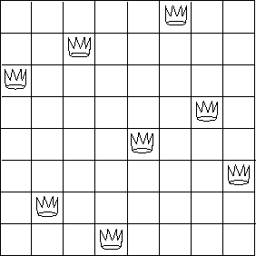
可以表示为(list 6 3 1 7 5 8 2 4)。
其中列表的第一个元素表示第8列的皇后所在的行,而列表的第二个元素表示第7列的皇后 所在的行,以此类推。
一个空棋盘可以使用'()表示:
;;; 42-empty-board.scm

(define empty-board '())
因为题目要求给出八皇后问题的所有解法,所以queens求出的最终结果将是一个
二维列表:(list (list 6 3 1 7 5 8 2 4) (list ...) (list ...) ...)。
添加皇后
添加皇后的工作由adjoin-position完成,它简单地将新皇后的行位置new-row添加到
列表的前端,因为列表中元素的位置指定了列的位置,所以参数k实际上是用不上的:
;;; 42-adjoin-position.scm

(define (adjoin-position new-row k rest-of-queens)
    (cons new-row rest-of-queens))
添加皇后的简单性是产生逆序列表的其中一个原因,另一个原因是,逆序列表会使得
接下来定义的safe?函数可以方便地从高到低检查棋盘的安全性。
过滤不安全的皇后
safe?以及它的辅助函数iter-check完成过滤不安全皇后的操作,对于一个给定的
新皇后行,它迭代地向棋盘的下方检查是否有已存在的皇后和新皇后的行发生冲突:
;;; 42-safe.scm

(define (safe? k position)
    (iter-check (car position)
                (cdr position)
                 1))

(define (iter-check row-of-new-queen rest-of-queens i)
	(if (null? rest-of-queens)  ; 下方所有皇后检查完毕,新皇后安全
		#t
		(let ((row-of-current-queen (car rest-of-queens)))
			(if (or (= row-of-new-queen row-of-current-queen)     ; 行碰撞
					(= row-of-new-queen (+ i row-of-current-queen))   ; 右下方碰撞
					(= row-of-new-queen (- row-of-current-queen i)))  ; 左下方碰撞
				#f
				(iter-check row-of-new-queen
					(cdr rest-of-queens)               ; 继续检查剩余的皇后
					(+ i 1))))))                       ; 更新步进值
比如说,当k为4,新皇后放在第5行的时候,产生这样一个检查序列
(o号表示皇后,x表示被检查的位置):
8                                           (safe? 4 (list 5 8 2 4))

7

6

5

4                   o

3                               o

2       o

1               o

    1   2   3   4   5   6   7   8

8                                           (iter-check 4 (list 5 8 2 4) 1)

7

6

5

4                   o

3               x   x   x       o

2       o

1               o

    1   2   3   4   5   6   7   8


8                                           (iter-check 5 (list 2 4) 2)

7

6

5

4                   o

3               x   x   x       o

2       o   x       x       x

1               o

    1   2   3   4   5   6   7   8

8                                           (iter-check 5 (list 4) 3)

7

6

5

4                   o

3               x   x   x       o

2       o   x       x       x

1       x       o   x           x

    1   2   3   4   5   6   7   8
生成八皇后的所有解
1 ]=> (load "42-queens.scm")

;Loading "42-queens.scm"...
;  Loading "p78-enumerate-interval.scm"... done
;  Loading "p83-flatmap.scm"...
;    Loading "p78-accumulate.scm"... done
;  ... done
;  Loading "42-safe.scm"... done
;  Loading "42-empty-board.scm"... done
;  Loading "42-adjoin-position.scm"... done
;... done
;Value: queens

1 ]=> (for-each (lambda (pos)
                    (begin
                        (display pos)
                        (newline)))
                (queens 8))

(4 2 7 3 6 8 5 1)
(5 2 4 7 3 8 6 1)
(3 5 2 8 6 4 7 1)
(3 6 4 2 8 5 7 1)
(5 7 1 3 8 6 4 2)
(4 6 8 3 1 7 5 2)
(3 6 8 1 4 7 5 2)
(5 3 8 4 7 1 6 2)
(5 7 4 1 3 8 6 2)
(4 1 5 8 6 3 7 2)
(3 6 4 1 8 5 7 2)
(4 7 5 3 1 6 8 2)
(6 4 2 8 5 7 1 3)
(6 4 7 1 8 2 5 3)
(1 7 4 6 8 2 5 3)
(6 8 2 4 1 7 5 3)
(6 2 7 1 4 8 5 3)
(4 7 1 8 5 2 6 3)
(5 8 4 1 7 2 6 3)
(4 8 1 5 7 2 6 3)
(2 7 5 8 1 4 6 3)
(1 7 5 8 2 4 6 3)
(2 5 7 4 1 8 6 3)
(4 2 7 5 1 8 6 3)
(5 7 1 4 2 8 6 3)
(6 4 1 5 8 2 7 3)
(5 1 4 6 8 2 7 3)
(5 2 6 1 7 4 8 3)
(6 3 7 2 8 5 1 4)
(2 7 3 6 8 5 1 4)
(7 3 1 6 8 5 2 4)
(5 1 8 6 3 7 2 4)
(1 5 8 6 3 7 2 4)
(3 6 8 1 5 7 2 4)
(6 3 1 7 5 8 2 4)
(7 5 3 1 6 8 2 4)
(7 3 8 2 5 1 6 4)
(5 3 1 7 2 8 6 4)
(2 5 7 1 3 8 6 4)
(3 6 2 5 8 1 7 4)
(6 1 5 2 8 3 7 4)
(8 3 1 6 2 5 7 4)
(2 8 6 1 3 5 7 4)
(5 7 2 6 3 1 8 4)
(3 6 2 7 5 1 8 4)
(6 2 7 1 3 5 8 4)
(3 7 2 8 6 4 1 5)
(6 3 7 2 4 8 1 5)
(4 2 7 3 6 8 1 5)
(7 1 3 8 6 4 2 5)
(1 6 8 3 7 4 2 5)
(3 8 4 7 1 6 2 5)
(6 3 7 4 1 8 2 5)
(7 4 2 8 6 1 3 5)
(4 6 8 2 7 1 3 5)
(2 6 1 7 4 8 3 5)
(2 4 6 8 3 1 7 5)
(3 6 8 2 4 1 7 5)
(6 3 1 8 4 2 7 5)
(8 4 1 3 6 2 7 5)
(4 8 1 3 6 2 7 5)
(2 6 8 3 1 4 7 5)
(7 2 6 3 1 4 8 5)
(3 6 2 7 1 4 8 5)
(4 7 3 8 2 5 1 6)
(4 8 5 3 1 7 2 6)
(3 5 8 4 1 7 2 6)
(4 2 8 5 7 1 3 6)
(5 7 2 4 8 1 3 6)
(7 4 2 5 8 1 3 6)
(8 2 4 1 7 5 3 6)
(7 2 4 1 8 5 3 6)
(5 1 8 4 2 7 3 6)
(4 1 5 8 2 7 3 6)
(5 2 8 1 4 7 3 6)
(3 7 2 8 5 1 4 6)
(3 1 7 5 8 2 4 6)
(8 2 5 3 1 7 4 6)
(3 5 2 8 1 7 4 6)
(3 5 7 1 4 2 8 6)
(5 2 4 6 8 3 1 7)
(6 3 5 8 1 4 2 7)
(5 8 4 1 3 6 2 7)
(4 2 5 8 6 1 3 7)
(4 6 1 5 2 8 3 7)
(6 3 1 8 5 2 4 7)
(5 3 1 6 8 2 4 7)
(4 2 8 6 1 3 5 7)
(6 3 5 7 1 4 2 8)
(6 4 7 1 3 5 2 8)
(4 7 5 2 6 1 3 8)
(5 7 2 6 3 1 4 8)
;Unspecified return value
练习 2.43
以下的八皇后程序运行极慢,原因是flatmap里写错交换嵌套映射和的顺序:
(define (queens board-size)
  (define (queen-cols k)
    (if (= k 0)
        (list empty-board)
        (filter
         (lambda (positions) (safe? k positions))
	 ;; next expression changed
         (flatmap
	  (lambda (new-row)
	    (map (lambda (rest-of-queens)
		   (adjoin-position new-row k rest-of-queens))
		 (queen-cols (- k 1))))
	  (enumerate-interval 1 board-size)))))
  (queen-cols board-size))
解释一下这么慢的原因。
queens函数对于每个棋盘(queen-cols k),使用enumerate-interval产生
board-size个棋盘。
而 Louis 的queens函数对于(enumerate-interval 1 board-size)的每个k,
都要产生(queen-cols (- k 1))个棋盘。
因此, Louis的queens函数的运行速度大约是原来queens函数的board-size倍,
也即是T * board-size。